The Locked Numerical Instantiation Standard for Constraint-Based Realization | Completeness, Identifiability, Simulation Readiness, and Empirical Adjudication in a Platform-Specific CBR Dossier

---

Abstract

This paper develops a locked numerical instantiation standard for Constraint-Based Realization (CBR), a candidate law-form for individual quantum outcome realization. CBR treats realization as a distinct explanatory target: probability weights possible outcomes, decoherence stabilizes records, and registration makes records operationally available, but none of these by itself supplies a law of which admissible outcome is realized. In canonical form, CBR represents realization as context-fixed constrained selection,

Φ∗C ∈ argmin{Φ ∈ 𝒜(C)} ℛ_C(Φ), up to ≃_C,

where C is the measurement context, 𝒜(C) is the admissible candidate class, ≃_C is operational equivalence, and ℛ_C is a realization-burden functional.

The aim of this paper is not to confirm CBR empirically, derive a universal realization law, or infer realization directly from data. Its purpose is narrower and more operational: to define when a platform-specific CBR instantiation is sufficiently specified to be simulated, audited, and prepared for empirical adjudication without post hoc alteration. The paper introduces a locked dossier standard requiring prior registration of the law-form objects, accessibility bridge, ordinary baseline, nuisance envelope, detectability threshold, endpoint functional, predicted endpoint, degeneracy operator, statistical rule, provenance certificates, validity gates, and verdict procedure. In this structure, the empirical target is not realization itself but a registered accessibility-critical endpoint: the predicted residual structure that remains after comparison with ordinary quantum, decoherence, detector, calibration, sampling, and nuisance effects.

The central contribution is a theorem spine connecting numerical completeness, endpoint identifiability, simulation readiness, and adjudication readiness. A platform-specific CBR instantiation is numerically complete only when all adjudication-relevant objects are fixed before endpoint interpretation. Its endpoint is identifiable only if the predicted CBR endpoint exceeds the registered decision threshold, T_CBR > Θ_c, and the predicted residual is not absorbed by the ordinary-degeneracy operator, Δ_CBR ∉ Deg_C. It is simulation-ready only when baseline-only, CBR-positive, strong-null, inconclusive, and degeneracy scenarios can be generated from the locked dossier without adding new primary test objects. It is adjudication-ready only when the critical-path objects have sufficient provenance and the locked statistical rule can issue a verdict from an observed endpoint comparison.

The framework distinguishes completion, simulation, support, failure, and inconclusive exposure. Numerical completeness does not imply empirical confirmation. Simulation can test detectability, false-support risk, false-failure risk, nuisance sensitivity, sampling adequacy, degeneracy behavior, and strong-null logic, but it does not adjudicate nature. Public-data reanalysis can motivate constraints or test design, but it is not decisive unless accessibility calibration, baseline modeling, nuisance accounting, endpoint reconstruction, degeneracy analysis, and statistical validity are adequate. The resulting standard makes a CBR platform instantiation test-ready in a disciplined sense: it specifies what must be locked, what can count as support, what would constitute failure, what remains inconclusive, and why post hoc rescue is not permitted.

---

SECTION 1. Introduction — From Law-Form to Computable Instantiation

The locked-dossier protocol specifies how a CBR test must be registered before data interpretation. It fixes the empirical endpoint, baseline model class, nuisance envelope, decision threshold, endpoint statistic, predicted endpoint, validity gates, statistical rule, and verdict rule. That protocol prevents post hoc rescue and anomaly hunting.

A further question remains: What exactly is being computed in a concrete platform?

A locked dossier can state that η, I_c, V_ℬ(η), B_𝓝(η), Θ_c, T_c, and T_CBR must be fixed. But a mathematically serious CBR instantiation must do more than list those objects. It must define how they are generated from a declared measurement context.

This paper provides that next step.

It constructs a platform-specific numerical instantiation of CBR in a record-accessibility interferometric context. The aim is not to prove CBR, not to report empirical confirmation, and not to define the final universal realization-burden functional. The aim is narrower and more technical: to show how a declared context C can generate a candidate class 𝒜(C), a computable platform-level burden proxy ℛ_C^plat, an accessibility bridge from η to the observable endpoint, a baseline model class 𝔅, a nuisance envelope B_𝓝(η), a decision threshold Θ_c, and a predicted endpoint T_CBR.

The governing pathway is:

C → 𝒜(C) → ℛ_C^plat → η bridge → Δ_CBR(η) → T_CBR.

This pathway is the paper’s central contribution. It moves CBR from locked empirical architecture to computable platform-specific instantiation.

1.1 The Problem

CBR’s canonical law-form is:

Φ∗C ∈ argmin{Φ ∈ 𝒜(C)} ℛ_C(Φ), up to ≃_C.

This expression supplies the formal structure of constrained selection. However, an empirical test requires platform-level objects that can be computed, bounded, simulated, or compared with data.

A critic can therefore ask: Given an actual interferometric context, how are 𝒜(C), ℛ_C^plat, η, I_c, 𝔅, V_ℬ(η), B_𝓝(η), Θ_c, T_c, and T_CBR obtained?

If those objects are not generated by registered rules, the model remains under-specified. If they are selected after data inspection, the analysis becomes exploratory. If they are too flexible, the model risks absorbing any outcome. If they are too narrow, it risks false support.

This paper addresses that problem by defining a numerical instantiation standard.

1.2 The Central Advancement

The paper’s central advancement is the construction of a computable platform-level CBR instantiation.

It provides:

a declared measurement context C,
a candidate-generation rule for 𝒜(C),
an operational equivalence relation ≃_C,
a computable burden proxy ℛ_C^plat,
an accessibility bridge from η to V_CBR(η),
a predicted residual Δ_CBR(η),
a predicted endpoint T_CBR,
a baseline model class 𝔅,
a nuisance envelope B_𝓝(η),
a decision threshold Θ_c,
and an identifiability rule governing when the predicted residual is distinguishable from ordinary baseline and nuisance behavior.

This is stronger than a checklist. It is a generative model of the registered test objects.

1.3 Scope

This paper is platform-specific.

It does not claim to define the final universal burden functional ℛ_C for all measurement contexts. Instead, it defines a registered platform-level burden proxy ℛ_C^plat sufficient for numerical modeling, simulation, and future empirical comparison in a declared record-accessibility interferometric context.

The distinction matters. A platform proxy is not a universal law. It is a controlled instantiation of the CBR law-form under a declared context and registered assumptions.

Accordingly, the paper’s claim is conditional: If a platform-specific CBR instantiation supplies a constructively generated candidate class, a computable burden proxy, a registered accessibility bridge, and a predicted endpoint, then it becomes numerically executable in that declared context.

1.4 Main Contribution

The paper contributes eight objects to the CBR empirical-execution sequence.

First, it gives a constructive rule for 𝒜(C).

Second, it defines a computable platform burden proxy ℛ_C^plat.

Third, it states how η enters the burden proxy nontrivially.

Fourth, it defines the bridge:

η → ℛ_C^plat → Φ∗_C(η) → V_CBR(η) → Δ_CBR(η).

Fifth, it defines a baseline model class 𝔅, not merely a single idealized baseline curve.

Sixth, it defines the nuisance envelope and critical nuisance bound.

Seventh, it defines endpoint congruence between T_c and T_CBR.

Eighth, it states the numerical-completeness, bridge-computability, and platform-executability conditions required before the model can be simulated or compared with data.

1.5 Principle — Computable Instantiation

A platform-specific CBR instantiation is computable only if every primary object in the pathway C → 𝒜(C) → ℛ_C^plat → η bridge → Δ_CBR(η) → T_CBR is defined by a registered functional rule before data interpretation.

This principle prevents the paper from mistaking notation for computation. Naming 𝒜(C), ℛ_C^plat, or T_CBR is not enough. The model must specify how those objects are generated, evaluated, and locked.

1.6 Transition

The first required object is the declared measurement context C. Without a fixed platform context, none of the numerical objects can be generated without discretion.

SECTION 2. Declared Platform Context C

A platform-specific numerical instantiation begins by fixing the measurement context C.

For this paper, C is a record-accessibility interferometric context. This includes delayed-choice, quantum eraser, which-path marking, wave-particle duality, or related interferometric arrangements in which an interference visibility observable is evaluated while outcome-defining record-accessibility is varied.

The context C is not merely a background description. It is the root object of the numerical model. It determines which candidates are admissible, which distinctions are operationally meaningful, how η is calibrated, which baseline model class is relevant, what nuisance sources must be bounded, and what data are sufficient for adjudication.

2.1 Platform Choice

The declared platform class is: record-accessibility interferometry.

This class is appropriate because it contains the basic ingredients needed for an accessibility-critical residual test: a visibility observable, a record-accessibility control variable, a standard quantum/decoherence baseline, ordinary detector and nuisance mechanisms, and a possible critical accessibility regime in which a registered CBR residual may be evaluated.

The platform may be instantiated through a specific delayed-choice, quantum eraser, which-path marking, or wave-particle duality arrangement. The present paper defines the numerical structure required for such a platform. A later empirical or public-data paper may instantiate it with a particular dataset.

2.2 Measurement Context C

Let C include all registered features needed to define the model:

state preparation,
interferometric alternatives,
record channel,
which-path or record marker,
record-accessibility control,
visibility readout,
timing window or coincidence rule where applicable,
detector model,
calibration protocol,
data-inclusion rule,
visibility estimator,
validity gates,
and statistical rule.

A change to any of these objects after data interpretation changes the test object. It may define a new dossier version, but it cannot rescue or reinterpret the original registered instantiation.

2.3 Why This Platform Is Suitable

The platform is suitable because it allows the core CBR empirical objects to be defined in a physically disciplined way.

The visibility observable supplies V_obs(η).

The record-accessibility control supplies η.

The ordinary quantum/decoherence account supplies the baseline model class 𝔅 and baseline curve V_ℬ(η).

Detector behavior, calibration uncertainty, phase drift, finite sampling, and environmental noise supply nuisance components for B_𝓝(η).

The critical accessibility region supplies I_c or N(η_c).

The registered CBR bridge supplies the predicted endpoint T_CBR.

Thus, the platform is suitable not because it proves CBR, but because it is rich enough to express the locked empirical structure.

2.4 Platform Limitation

This model does not apply to all quantum measurements.

It applies only to the declared platform class C. A different measurement context would require its own candidate-generation rule, burden proxy, accessibility bridge, baseline model class, nuisance envelope, endpoint statistic, and predicted endpoint.

This limitation is a strength rather than a weakness. CBR’s empirical claims must be context-fixed. A platform-specific instantiation should not pretend to be universal.

2.5 Definition — Declared Numerical Context

A declared numerical context C is a fixed record-accessibility interferometric context containing enough operational structure to generate 𝒜(C), ≃_C, ℛ_C^plat, η, I_c, 𝔅, V_ℬ(η), B_𝓝(η), T_c, and T_CBR under registered rules.

This definition makes C the root object of the numerical model.

2.6 Context Completeness Condition

A declared context is complete for numerical execution only if it supplies enough information to determine:

the preliminary candidate space Ω_C,
the admissibility filters generating 𝒜(C),
the operational equivalence relation ≃_C,
the domain of ℛ_C^plat,
the calibration of η,
the visibility-response map V(Φ, C),
the baseline model class 𝔅,
and the data-adequacy requirements for T_c.

If any of these are missing, the context may still be conceptually meaningful, but it is not yet numerically executable.

2.7 Transition

Once C is fixed, the paper can construct the admissible candidate class 𝒜(C). Without a constructive candidate class, the burden functional would have no well-defined domain.

SECTION 3. Candidate-Generation Rule for 𝒜(C)

Let 𝒜(C) denote the platform-generated admissible candidate class for the declared context C.

The purpose of this section is to make 𝒜(C) constructive rather than nominal. The candidate class cannot be a vague set of possible outcomes. It must be generated by registered filters applied to a declared platform candidate space.

3.1 Candidate Space and Admissibility

Let Ω_C denote the preliminary platform candidate space: the set of candidate descriptions that can be formulated for the declared context C before admissibility filters are applied.

A candidate Φ ∈ Ω_C belongs to 𝒜(C) only if it satisfies all registered admissibility filters.

The admissible class is therefore not:

all imaginable possibilities,
all mathematically writable alternatives,
or all post hoc candidate descriptions compatible with the observed result.

It is the class of candidates that survive the registered constraints of the context before data interpretation.

3.2 Candidate Filters

A candidate Φ is admissible only if it satisfies the following filters.

Context compatibility.
Φ must be defined within the fixed measurement context C.

Instrument compatibility.
Φ must respect the registered preparation, measurement, record, and visibility-readout structure.

Record-structure compatibility.
Φ must specify how outcome-defining record information is represented within the platform.

Visibility-response definability.
Φ must determine, or be compatible with, a defined visibility response V_Φ(η).

Operational evaluability.
Φ must be evaluable by the registered endpoint statistic and statistical rule.

Born-discipline constraint.
Φ must not arbitrarily violate the ensemble-level quantum probability structure unless the instantiation explicitly registers a scoped deviation.

Decoherence-baseline compatibility.
Φ must respect the registered standard quantum/decoherence baseline structure except where the CBR instantiation explicitly predicts a residual.

Burden-evaluability.
Φ must be evaluable by ℛ_C^plat.

Non-post-hoc definability.
Φ must be specified before data interpretation.

These filters are not decorative. They prevent 𝒜(C) from becoming an adjustable possibility space.

3.3 Candidate-Generation Rule

The candidate-generation rule is:

𝒜(C) = {Φ ∈ Ω_C : F_i(Φ, C) = 1 for every registered admissibility filter F_i}.

Equivalently, a candidate is admissible only if it passes all registered filters:

Φ ∈ 𝒜(C) ⇔ Φ ∈ Ω_C and F₁(Φ, C) = ⋯ = F_n(Φ, C) = 1.

This makes 𝒜(C) a generated object, not an interpretive label.

3.4 Candidate Evaluability Condition

The generated candidate class must be evaluable.

For every Φ ∈ 𝒜(C), the following must be defined:

ℛ_C^plat(Φ; η),
V_Φ(η) or the rule by which Φ determines visibility,
the operational equivalence class of Φ under ≃_C,
and the endpoint contribution of Φ under the registered endpoint functional.

If any candidate admitted into 𝒜(C) cannot be evaluated by the burden proxy or visibility-response map, then the candidate-generation rule is incomplete.

3.5 Operational Equivalence ≃_C

The operational equivalence relation ≃_C identifies candidates that differ formally but not operationally within the declared test.

Define:

Φ₁ ≃_C Φ₂

if Φ₁ and Φ₂ are indistinguishable under the registered observables, uncertainty convention, endpoint statistic, and statistical rule.

For the present platform, a sufficient operational-equivalence criterion is:

Φ₁ ≃_C Φ₂ if T_c(Φ₁) and T_c(Φ₂) are indistinguishable under the registered statistical rule.

If the endpoint is morphology-sensitive, operational equivalence must also include morphology equivalence under the registered comparison rule.

The selection object is therefore 𝒜(C)/≃_C, not the unquotiented candidate list.

3.6 Candidate-Class Lock Rule

The candidate class cannot be expanded, narrowed, re-filtered, or reinterpreted after data interpretation.

If new filters are added, old filters are removed, or candidate definitions are changed after observing V_obs(η) or r(η), the original numerical instantiation has not been preserved. A new dossier version has been created.

This rule prevents candidate engineering after the outcome.

Proposition 1 — Candidate-Class Constructibility

For a platform-specific CBR instantiation to be numerically adjudicable, 𝒜(C) must be generated by registered admissibility filters applied to a declared platform candidate space Ω_C before data interpretation.

Proof Sketch

The burden proxy ℛ_C^plat requires a domain. If 𝒜(C) is not generated by registered rules, then the domain of minimization can be changed after the result. If the domain can be changed after the result, the selection rule is not exposed to failure. Therefore, numerical adjudication requires a pre-data candidate-generation rule.

Corollary — Candidate Evaluability

A generated candidate class is numerically complete only if every candidate Φ ∈ 𝒜(C) is evaluable by ℛ_C^plat, classifiable under ≃_C, and connected to the registered visibility-response map.

Proof Sketch

A candidate that cannot be evaluated by ℛ_C^plat cannot enter the minimization rule. A candidate that cannot be classified under ≃_C cannot be compared at the operational level. A candidate that cannot be connected to visibility cannot contribute to T_CBR. Therefore, candidate admissibility requires evaluability, not merely formal inclusion.

3.7 Transition

With 𝒜(C) defined as a generated and evaluable admissible class, the next step is to define the computable burden proxy that orders candidates within 𝒜(C)/≃_C.

SECTION 4. Computable Platform Burden Proxy ℛ_C^plat

CBR’s canonical law-form requires a realization-burden functional:

Φ∗C ∈ argmin{Φ ∈ 𝒜(C)} ℛ_C(Φ), up to ≃_C.

For a platform-specific numerical instantiation, this paper defines a computable burden proxy:

ℛ_C^plat(Φ; η).

This proxy is not claimed to be the final universal burden functional for CBR. It is the registered platform-level functional used to generate a numerical prediction in the declared context C.

The proxy must satisfy five requirements.

It must be defined on 𝒜(C)/≃_C.
It must be computable before data interpretation.
It must allow η to enter nontrivially.
It must be stable under the registered coefficient and normalization rules.
It must generate a predicted endpoint T_CBR through a registered bridge.

4.1 Proposed Functional Form

A platform-level burden proxy may be represented as:

ℛ_C^plat(Φ; η) = αΞ_C(Φ; η) + βΩ_C(Φ) + γΛ_C(Φ).

Here:

Ξ_C(Φ; η) is the accessibility burden term.
Ω_C(Φ) is the baseline/decoherence consistency term.
Λ_C(Φ) is the stability, non-adaptivity, or complexity-control term.
α, β, γ are registered coefficients.

This expression is a platform-specific modeling form. It should not be presented as the final universal CBR law unless a later paper proves that status.

4.2 Principle — Burden-Term Definition Obligation

A platform-specific burden proxy ℛ_C^plat is not numerically complete merely because its terms are named. Each term Ξ_C, Ω_C, and Λ_C must be defined by a registered functional rule with a specified domain, range, normalization convention, coefficient rule, and data-independence condition. If any term cannot be evaluated for every Φ ∈ 𝒜(C), the numerical instantiation is incomplete rather than adjudicative.

This principle is essential. Without it, ℛ_C^plat would be a notation scheme rather than a computable object.

4.3 Accessibility Term Ξ_C

The term Ξ_C(Φ; η) represents the part of the burden proxy that changes as record-accessibility changes.

It is the term through which η enters the realization-burden structure nontrivially.

For this term to be admissible, the paper must specify:

the domain of Ξ_C,
the range of Ξ_C,
how η is calibrated,
how η enters Ξ_C,
how Ξ_C changes candidate ordering,
whether Ξ_C predicts a magnitude, morphology, or transition behavior,
how Ξ_C is normalized relative to the other terms,
and how its contribution is locked before data interpretation.

Without this term, η may be descriptive but not dynamically relevant to the registered CBR instantiation.

4.4 Baseline / Decoherence Consistency Term Ω_C

The term Ω_C(Φ) penalizes candidates that violate the registered ordinary baseline structure without a declared CBR residual.

Its role is not to force CBR to reduce to standard quantum/decoherence behavior. Its role is to prevent arbitrary residual fitting.

For this term to be admissible, the paper must specify:

the domain of Ω_C,
the range of Ω_C,
which baseline constraints it enforces,
how it interacts with the baseline model class 𝔅,
how ordinary decoherence consistency is represented,
how deviations are allowed only when registered as a CBR endpoint,
and how Ω_C is normalized.

A candidate may predict an accessibility-critical residual only if that residual is registered as part of the instantiation and later tested against 𝔅, B_𝓝(η), and Θ_c.

Thus, Ω_C enforces ordinary-physics discipline without eliminating the possibility of a CBR-specific endpoint.

4.5 Stability / Non-Adaptivity Term Λ_C

The term Λ_C(Φ) penalizes instability, excessive flexibility, or post hoc adjustability.

A candidate should not become favorable merely because it can be tuned to match whatever residual appears. Λ_C encodes the requirement that the candidate’s structure be stable under the registered modeling assumptions.

For this term to be admissible, the paper must specify:

the domain of Λ_C,
the range of Λ_C,
which forms of flexibility it penalizes,
how it distinguishes legitimate platform parameters from post hoc tuning,
how it is normalized,
and how it remains independent of the observed residual.

This term helps prevent overfitting and failure rescue.

4.6 Coefficient Fixity

The coefficients α, β, γ must be fixed by registered rules before data interpretation.

Permitted sources include:

normalization conventions,
platform calibration,
prior theoretical commitments,
simulation conventions,
sensitivity constraints,
or declared illustrative modeling assumptions.

Forbidden sources include:

outcome fitting,
post hoc residual matching,
coefficient adjustment after failure,
or tuning to produce support.

If coefficient values are illustrative or simulated, they must be labeled as such. They must not be presented as measured or empirically validated.

4.7 Selection Rule

The platform selection rule is:

Φ∗C(η) ∈ argmin{Φ ∈ 𝒜(C)} ℛ_C^plat(Φ; η), up to ≃_C.

The dependence on η does not mean that the model may adjust itself after the data are known. It means that, for each registered value of record-accessibility, the platform proxy orders admissible candidates according to a fixed functional rule.

4.8 Burden-Proxy Lock Rule

The terms Ξ_C, Ω_C, Λ_C, the coefficients α, β, γ, normalization rules, candidate domain, and data-independence conditions must be fixed before endpoint evaluation.

Any change to the burden proxy after data interpretation creates a new numerical instantiation. It does not rescue or revise the verdict of the prior version.

Proposition 2 — Burden-Proxy Computability

A platform-specific CBR model is numerically executable only if its burden proxy ℛ_C^plat is defined on 𝒜(C)/≃_C, computable under registered rules, and fixed before data interpretation.

Proof Sketch

The selection rule requires a functional ordering over admissible candidates. If the functional is undefined, the selection rule cannot be evaluated. If the functional is not computable, the model cannot generate a numerical endpoint. If the functional is changed after data interpretation, the model is no longer locked. Therefore, numerical execution requires a fixed computable burden proxy.

Corollary — Named Terms Are Insufficient

A platform burden proxy whose terms are named but not mathematically evaluable is incomplete.

Proof Sketch

A term such as Ξ_C, Ω_C, or Λ_C contributes to ℛ_C^plat only if it can be evaluated for admissible candidates. If it cannot be evaluated, then the burden proxy cannot order 𝒜(C)/≃_C. Therefore, named but unevaluable terms do not yet define a numerical model.

4.9 Transition

Once the burden proxy is defined, the model must state how record-accessibility η enters that proxy and how the resulting candidate selection produces a visibility-level prediction.

SECTION 5. Accessibility Bridge: η → ℛ_C^plat → Δ_CBR(η)

The accessibility bridge is the central connection between the CBR law-form and the measurable endpoint.

The bridge must show how record-accessibility η enters ℛ_C^plat, how the minimizer Φ∗_C(η) determines a predicted visibility response, and how that response generates a predicted residual Δ_CBR(η).

Without this bridge, the platform model may be formally defined, but it is not yet empirically exposed.

5.1 Operational Definition of η

Let η denote the operational record-accessibility variable.

η is not consciousness, subjective awareness, observer knowledge, human attention, or metaphysical observation. It is a platform-calibrated measure of accessible outcome-defining record information.

In a record-accessibility interferometric context, η may be instantiated through:

which-path distinguishability,
record-retention probability,
marker strength,
eraser accessibility,
path-knowledge parameter,
coincidence-conditioned accessibility,
or another registered accessibility proxy.

The chosen proxy must be specified before residual evaluation.

5.2 η Calibration

The platform model must define:

the range of η,
the resolution of η,
the uncertainty in η,
the calibration method,
the sampling requirements,
the relationship between η and the physical accessibility-control mechanism,
and the effect of η uncertainty on T_CBR and T_c.

If η is only qualitatively described, the instantiation is incomplete. If η is reconstructed after seeing the residual, the analysis is exploratory.

5.3 Critical Accessibility Regime

The model must declare a critical accessibility regime:

I_c = [η₁, η₂]

or:

N(η_c) = {η : |η − η_c| ≤ δ}.

The critical regime is the region where the platform model predicts the accessibility-sensitive endpoint to be strongest, most identifiable, or most decision-relevant.

The justification may be theoretical, numerical, bridge-based, or platform-specific, but it must be fixed before residual inspection.

5.4 Bridge Equation

The numerical bridge is:

η → ℛ_C^plat(Φ; η) → Φ∗_C(η) → V_CBR(η) → Δ_CBR(η).

Define the CBR-predicted visibility response:

V_CBR(η) = V(Φ∗_C(η), C),

where V is the registered visibility-response map for the platform.

Define the predicted residual:

Δ_CBR(η) = V_CBR(η) − V_ℬ(η).

Then define the predicted endpoint:

T_CBR = 𝒯[Δ_CBR(η), η ∈ I_c],

where 𝒯 is the registered endpoint functional.

This is the core numerical pathway of the paper.

5.5 Computability Condition

The bridge η → ℛ_C^plat → Φ∗_C(η) → V_CBR(η) → Δ_CBR(η) → T_CBR is complete only if every arrow is defined by a registered map. If any arrow is interpretive rather than functional, the model remains schematic rather than numerically executable.

This condition prevents the bridge from functioning merely as a conceptual diagram. A numerical instantiation must specify the maps, not only their names.

5.6 Bridge Completeness

The accessibility bridge is complete only if it specifies:

how η enters ℛ_C^plat,
how η can change candidate ordering,
how Φ∗_C(η) determines V_CBR(η),
how Δ_CBR(η) is generated,
which endpoint functional 𝒯 is applied,
how T_CBR is computed,
and what absence of the endpoint would count as registered failure.

If any of these are missing, the bridge is incomplete.

5.7 Bridge Nontriviality

η must enter the burden proxy nontrivially.

A merely cosmetic η-dependence is insufficient. The model must state whether η changes candidate ordering, endpoint magnitude, endpoint morphology, or detectability status.

If η does not affect ℛ_C^plat or T_CBR, then the model does not generate an accessibility-critical prediction.

Proposition 3 — Accessibility-Bridge Completeness

A platform-specific CBR instantiation generates a predicted accessibility-critical residual only if η enters ℛ_C^plat nontrivially, the selected candidate Φ∗_C(η) determines a registered visibility response V_CBR(η), and the predicted residual Δ_CBR(η) yields a computable endpoint T_CBR under the registered endpoint functional.

Proof Sketch

The accessibility-critical residual is an empirical endpoint, not the law itself. To generate that endpoint, the law-form must be connected to an observable. If η does not enter the burden proxy, accessibility variation cannot affect the predicted endpoint. If the selected candidate does not determine a visibility response, no residual can be computed. If no endpoint functional is registered, no prediction can be adjudicated. Therefore, bridge completeness requires nontrivial η entry, a visibility-response map, and a computable T_CBR.

Theorem 1 — Platform Executability

A declared CBR platform model is executable only if 𝒜(C) is constructively generated, ℛ_C^plat is computable on 𝒜(C)/≃_C, η enters ℛ_C^plat nontrivially, Φ∗_C(η) determines V_CBR(η), Δ_CBR(η) is defined relative to V_ℬ(η), and T_CBR is obtained by applying the registered endpoint functional to Δ_CBR(η) over I_c.

Proof Sketch

A platform model is executable only if each step from context to prediction is defined. The context C generates 𝒜(C). The burden proxy ℛ_C^plat orders candidates in 𝒜(C)/≃_C. Nontrivial η-dependence allows accessibility variation to affect the selection structure. The selected candidate must determine a visibility response V_CBR(η). The residual Δ_CBR(η) must be defined relative to the registered baseline V_ℬ(η). The endpoint T_CBR must then be computed by the registered endpoint functional over the declared critical regime. If any step is missing, the platform model remains schematic. Therefore, all listed conditions are required for executability.

5.8 Transition

The bridge defines the CBR-side prediction. The next required object is the ordinary baseline model class 𝔅, which determines what standard quantum/decoherence/nuisance physics can explain before any CBR-specific residual is considered.

SECTION 6. Baseline Model Class 𝔅

The baseline model class defines what ordinary quantum, decoherence, detector, calibration, sampling, and platform effects can explain before any CBR-specific residual is considered. It is therefore one of the central safeguards against false support.

CBR does not receive support by outperforming an idealized or artificially narrow baseline. A CBR residual becomes relevant only after ordinary physics has been given its strongest registered expression in the declared platform context.

6.1 Definition

Let:

𝔅 = {V_ℬ(η; θ) : θ ∈ Θ_ℬ}

where Θ_ℬ is the registered ordinary-physics parameter space.

Each member of 𝔅 is a candidate baseline visibility function representing standard quantum/decoherence/nuisance-compatible behavior in the declared context C. The selected or bounded baseline visibility curve V_ℬ(η) must be obtained from 𝔅 by a registered selection, fitting, calibration, or bounding rule fixed before endpoint evaluation.

Thus, V_ℬ(η) is not an arbitrary curve. It is the baseline consequence of a registered model class.

6.2 Included Ordinary Effects

The baseline model class should include all ordinary effects that the platform can justify as relevant, including:

standard quantum visibility prediction,
decoherence,
detector inefficiency,
dark counts,
loss,
phase drift,
finite sampling,
calibration uncertainty,
alignment uncertainty,
visibility-estimator uncertainty,
environmental noise,
postselection effects where applicable,
and timing or coincidence-window effects where applicable.

The exact list is platform-specific. The rule is not that every possible effect must be included in every model. The rule is that no legitimate ordinary effect may be excluded merely to make a residual appear more CBR-relevant.

6.3 Baseline Guardrail

The baseline model class must be disciplined in both directions.

It must be broad enough to include legitimate standard quantum/decoherence/nuisance explanations.

It must not be so broad that it can absorb any possible residual by construction.

A baseline class that is too narrow creates false support.
A baseline class that is too elastic prevents possible failure.

The valid baseline class is therefore:

strong enough to protect against false attribution, but constrained enough to preserve adjudication.

6.4 Baseline Selection Rule

The dossier must specify how V_ℬ(η) is selected, fitted, calibrated, or bounded from 𝔅.

Permissible baseline-selection modes include:

fixed-parameter baseline,
calibrated-parameter baseline,
bounded-envelope baseline,
held-out-fit baseline,
control-regime-fit baseline,
or published-parameter baseline.

Whichever mode is used, it must be registered before endpoint evaluation.

The selection rule must specify:

the allowed parameter space Θ_ℬ,
which parameters are fixed, calibrated, fitted, or bounded,
which data, if any, may be used to fit baseline parameters,
whether held-out or control-region data are required,
how baseline uncertainty propagates into the nuisance envelope,
how baseline uncertainty is distinguished from nuisance uncertainty,
and when a candidate residual is considered absorbable by 𝔅.

6.5 Principle — Parameter Provenance

Every numerical quantity entering 𝔅, V_ℬ(η), B_𝓝(η), B_c, ε_detect, Θ_c, T_c, and T_CBR must be assigned a registered provenance label before data interpretation.

Permissible labels include:

measured,
published,
calibrated,
derived,
simulated,
illustrative,
assumed,
or required for future testing.

A quantity with unclear provenance cannot support adjudication. If a value is illustrative, it must not be presented as measured. If a value is simulated, it must not be presented as empirical. If a value is required for future testing, it must not be treated as already available.

This principle prevents numerical modeling from acquiring false empirical authority.

6.6 Baseline Anti-Overfitting Rule

The baseline model class 𝔅 may not be expanded, refit, re-parameterized, or reinterpreted after inspecting the residual curve:

r(η) = V_obs(η) − V_ℬ(η)

in a way that changes the registered verdict.

If a residual is absorbed only by adding new baseline terms, changing the fitting rule, expanding Θ_ℬ, altering the validation standard, or relabeling a CBR-like feature as ordinary behavior after data interpretation, then the original test object has changed.

A revised baseline may be scientifically useful. It may define a new dossier version. It does not rescue the prior version.

The locked rule is:

A new baseline creates a new test object. It does not save the old one.

6.7 Definition — Baseline Degeneracy

A predicted residual Δ_CBR(η) is baseline-degenerate if there exists an allowed baseline member:

V_ℬ(η; θ′) ∈ 𝔅

such that the predicted CBR residual becomes indistinguishable from ordinary baseline behavior under the registered endpoint functional and statistical rule.

Equivalently, Δ_CBR(η) is baseline-degenerate if the CBR-predicted endpoint can be absorbed by an allowed change of baseline parameters without violating the registered baseline-selection rule.

A baseline-degenerate predicted endpoint cannot support CBR, even if it is mathematically defined. It may still motivate better modeling, but it is not identifiable as a CBR endpoint.

6.8 Baseline Adequacy Condition

A baseline class is adequate only if it can answer the following question in the declared context:

What visibility behavior should be expected across I_c or N(η_c) if no CBR-specific accessibility-critical residual is present?

If 𝔅 cannot answer this question with sufficient precision, then the test cannot adjudicate CBR support or failure. A positive-looking residual may be ordinary under-modeling. A null result may be uninterpretable because the expected baseline itself is not stable.

Proposition 4 — Baseline Adequacy

A platform-specific CBR residual test is baseline-adequate only if 𝔅 is registered before endpoint evaluation, includes the strongest ordinary platform explanations that can be justified, supplies or bounds V_ℬ(η) across the declared critical regime, uses provenance-labeled numerical quantities, remains non-adaptive after residual inspection, and does not render the predicted CBR endpoint baseline-degenerate.

Proof Sketch

The accessibility-critical residual is defined relative to V_ℬ(η). If the baseline is weak, a residual may appear only because ordinary physics was under-modeled. If the baseline is too elastic, no residual could ever survive. If the baseline is changed after the residual is known, the verdict applies to a different object. If the predicted residual is degenerate with an allowed baseline parameter shift, the endpoint cannot be identified as CBR-relevant. Therefore, baseline adequacy requires a strong, bounded, registered, provenance-labeled, non-adaptive, non-degenerate model class.

6.9 Transition

The baseline model class defines ordinary expected visibility. The next object defines how much ordinary deviation around that baseline can be absorbed without counting as CBR support.

SECTION 7. Nuisance Envelope and Critical Bound

The nuisance envelope specifies the ordinary non-CBR deviations from the registered baseline that the platform can absorb. It prevents CBR from treating detector drift, calibration uncertainty, finite sampling, phase instability, or model uncertainty as evidence for a realization-law endpoint.

The nuisance envelope is therefore not an afterthought. It is part of the empirical object being tested.

7.1 Definition

Let B_𝓝(η) be the registered nuisance envelope around V_ℬ(η).

It bounds deviations attributable to ordinary non-CBR sources in the declared platform context. These may include:

detector drift,
calibration uncertainty,
decoherence-model uncertainty,
phase instability,
sampling variation,
background counts,
alignment errors,
η uncertainty,
visibility-estimator uncertainty,
timing-window uncertainty,
postselection uncertainty,
and finite-count effects.

A residual inside the nuisance envelope is not CBR support. It is ordinary platform uncertainty.

7.2 Relation to Baseline Uncertainty

The nuisance envelope must include or explicitly coordinate with uncertainty in the baseline model class 𝔅.

If baseline uncertainty is represented separately from B_𝓝(η), the dossier must specify how both enter the decision rule. If baseline uncertainty is absorbed into B_𝓝(η), the envelope must state that explicitly.

The test cannot double-count uncertainty to make failure impossible, and it cannot omit uncertainty to manufacture support.

7.3 Critical Nuisance Bound

For endpoint adjudication inside the declared critical regime, the dossier must define a critical nuisance bound.

A standard form is:

B_c = sup_{η ∈ I_c} B_𝓝(η).

If the endpoint uses N(η_c) rather than I_c, then:

B_c = sup_{η ∈ N(η_c)} B_𝓝(η).

For normalized, integrated, model-comparison, or morphology-sensitive endpoints, B_c must be defined in the corresponding registered endpoint units.

This condition is essential. A nuisance bound expressed in pointwise visibility units cannot automatically be used for an integrated, normalized, or morphology-sensitive endpoint unless a registered transformation maps it into the same endpoint space.

7.4 Principle — Endpoint-Units Consistency

B_c, ε_detect, Θ_c, T_c, and T_CBR must be expressed in the same registered endpoint units.

A pointwise visibility nuisance bound cannot adjudicate an integrated, normalized, morphology-sensitive, or model-comparison endpoint unless a registered transformation maps it into the same endpoint space.

If the endpoint statistic is:

a supremum residual, then B_c, ε_detect, Θ_c, T_c, and T_CBR must be expressed in supremum-residual units;
a normalized statistic, they must be expressed in normalized units;
an integrated statistic, they must be expressed in integrated-endpoint units;
a morphology-sensitive statistic, they must be expressed in the registered morphology-comparison units;
a model-comparison statistic, they must be expressed in the registered model-comparison scale.

Without endpoint-units consistency, the comparison among T_c, T_CBR, and Θ_c is not adjudicative.

7.5 Nuisance Construction Rule

The dossier must specify how B_𝓝(η) is constructed.

It must state:

which nuisance sources are included,
how each source is estimated or bounded,
the provenance label for each nuisance quantity,
how uncertainties are propagated,
whether nuisance terms are added linearly, in quadrature, by envelope maximization, or by another registered rule,
what confidence or error-control convention is used,
how η uncertainty enters the envelope,
how baseline uncertainty interacts with the envelope,
and how B_c is derived from B_𝓝(η) in endpoint-compatible units.

If these rules are missing, the nuisance envelope is not numerically adjudicative.

7.6 Definition — Baseline/Nuisance Degeneracy

A predicted residual Δ_CBR(η) is baseline/nuisance-degenerate if there exists an allowed baseline member V_ℬ(η; θ′) ∈ 𝔅, or an allowed nuisance deformation within B_𝓝(η), such that the predicted endpoint becomes indistinguishable from ordinary behavior under the registered endpoint functional and statistical rule.

In that case, the predicted residual may be mathematically defined, but it is not empirically identifiable as CBR-relevant.

A degenerate predicted endpoint cannot support CBR. It may indicate that the platform, endpoint statistic, nuisance model, or predicted morphology is insufficiently discriminating.

7.7 Nuisance Anti-Rescue Rule

B_𝓝(η) and B_c cannot be widened after data interpretation in order to absorb a residual, avoid support, or prevent failure.

Such widening may motivate a revised nuisance model. It may define a new dossier version. It does not alter the verdict of the original locked version.

The rule is:

A new nuisance envelope creates a new test object. It does not rescue the old one.

7.8 Nuisance Adequacy Condition

The nuisance envelope must be conservative enough to absorb ordinary platform uncertainty, but not so broad that it eliminates adjudication.

Too narrow creates false support.
Too broad creates non-falsifiability.

A valid nuisance envelope is therefore:

ordinary-effect complete, uncertainty-explicit, endpoint-compatible, provenance-labeled, non-degenerate, and non-adaptive.

Proposition 5 — Nuisance Adequacy

A nuisance envelope is adequate for a CBR residual test only if B_𝓝(η) is registered before endpoint evaluation, bounds ordinary non-CBR deviations across the declared critical regime, yields a critical nuisance bound B_c in the units of the endpoint statistic, uses provenance-labeled numerical quantities, does not make the predicted endpoint baseline/nuisance-degenerate, and cannot be widened after residual inspection to change the verdict.

Proof Sketch

A residual cannot support CBR if it lies within ordinary nuisance. A strong null cannot be established if nuisance bounds are undefined or unstable. If nuisance is widened after the result, the tested object changes. If nuisance is expressed in units incompatible with the endpoint statistic, the decision threshold is not meaningful. If the predicted endpoint is degenerate with nuisance, it cannot be identified as CBR-relevant. Therefore, nuisance adequacy requires a pre-registered envelope, endpoint-compatible critical bound, provenance discipline, non-degeneracy, and an anti-rescue rule.

7.9 Transition

The nuisance bound defines what ordinary deviations can absorb. The test also requires a detectability margin specifying how large a residual must be before the platform can distinguish it from baseline-plus-nuisance behavior.

SECTION 8. Detectability and Decision Threshold

The detectability threshold specifies whether the platform is capable of distinguishing a CBR-relevant endpoint from ordinary baseline-plus-nuisance behavior. It prevents a null result from being mistaken for failure when the predicted effect was below the platform’s sensitivity.

Detectability is not a rhetorical claim that an effect is “large enough.” It is a registered numerical condition expressed in the same endpoint units as T_c, T_CBR, and B_c.

8.1 Detectability Threshold

Let ε_detect be the registered minimum detectable endpoint separation.

It must be defined in the same units as the endpoint statistic T_c and the predicted endpoint T_CBR. For a pointwise visibility endpoint, ε_detect may be expressed in visibility units. For a normalized, integrated, model-comparison, or morphology-sensitive endpoint, it must be expressed in the corresponding registered endpoint units.

The detectability threshold must be based on:

sampling density,
visibility resolution,
η uncertainty,
detector sensitivity,
systematic uncertainty,
statistical power,
endpoint morphology where applicable,
and the registered confidence or error-control convention.

Every numerical component entering ε_detect must carry a provenance label: measured, published, calibrated, derived, simulated, illustrative, assumed, or required for future testing.

8.2 Decision Threshold

The nuisance bound and detectability threshold combine into the registered decision threshold:

Θ_c = B_c + ε_detect.

This threshold is the minimum endpoint separation required for adjudication inside the declared critical accessibility regime.

It is not a visual margin. It is the registered boundary between residuals that remain absorbable by baseline-plus-nuisance behavior and residuals that exceed the platform’s ordinary allowance.

8.3 Endpoint-Units Discipline

The expression:

Θ_c = B_c + ε_detect

is meaningful only if B_c and ε_detect are expressed in the same registered endpoint units.

The comparison:

T_c > Θ_c

is meaningful only if T_c is expressed in those same units.

The comparison:

T_CBR > Θ_c

is meaningful only if T_CBR is expressed in those same units.

If endpoint-units consistency fails, the test is incomplete rather than adjudicative.

8.4 Detectability Condition

For registered failure to be possible, the predicted CBR endpoint must satisfy:

T_CBR > Θ_c.

If:

T_CBR ≤ Θ_c,

then the predicted endpoint is not distinguishable from the registered baseline-plus-nuisance-and-detectability allowance. In that case, a null result cannot fail the instantiation. The correct status is inconclusive for failure.

This protects CBR from unfair failure and protects the test from overclaiming.

8.5 Support Condition

For registered support to be possible, the observed endpoint must satisfy:

T_c > Θ_c

under valid conditions, and must match the registered residual morphology where applicable.

This condition is necessary but not automatically sufficient. Support also requires baseline separation, nuisance separation, non-degeneracy, valid η calibration, data adequacy, and satisfaction of the registered statistical rule and validity gates.

8.6 Detectability Registration

The dossier must specify:

how ε_detect is computed,
which uncertainty sources enter it,
the provenance label for each numerical input,
the power requirement for detecting T_CBR,
the sample size or η-density requirement,
the visibility-resolution requirement,
the endpoint-specific unit convention,
and the conditions under which detectability is considered achieved.

If ε_detect is not specified, the model is incomplete. If it is changed after data interpretation, the test object changes.

Proposition 6 — Detectability Discipline

A CBR test can fail a registered instantiation only if the predicted endpoint exceeds the registered decision threshold Θ_c, all threshold components are expressed in the same registered endpoint units, and the platform satisfies the registered sensitivity, sampling, calibration, and statistical conditions required to detect that endpoint.

Proof Sketch

Failure requires the absence of a predicted detectable endpoint. If T_CBR ≤ Θ_c, the predicted endpoint is not detectable under the registered conditions. If the threshold quantities are not expressed in the same endpoint units, the comparison is not meaningful. If the platform fails to satisfy the registered sensitivity conditions, the endpoint may be absent only because the test could not reveal it. Therefore, failure requires T_CBR > Θ_c, endpoint-units consistency, and achieved detectability.

8.7 Transition

The decision threshold prepares the model for endpoint adjudication. The next section defines the observed endpoint statistic T_c and the predicted endpoint T_CBR that are compared against Θ_c.

SECTION 9. Endpoint Statistic T_c and Predicted Endpoint T_CBR

The endpoint statistic is the rule that converts residual structure into an adjudicative quantity. It is the point at which the platform model becomes testable.

The key distinction is between the observed endpoint and the predicted endpoint.

T_c is computed from observed data.
T_CBR is generated by the registered CBR platform model.

A locked test requires both.

9.1 Observed Endpoint Statistic

Define:

T_c = 𝒯[V_obs(η) − V_ℬ(η), η ∈ I_c].

Here 𝒯 is the registered endpoint functional.

Possible endpoint functionals include:

supremum residual,
normalized supremum residual,
integrated residual,
localized kink statistic,
slope-change statistic,
curvature statistic,
morphology-sensitive statistic,
or model-comparison statistic.

For example:

T_c = sup_{η ∈ I_c} |V_obs(η) − V_ℬ(η)|

or:

T_c = sup_{η ∈ I_c} |V_obs(η) − V_ℬ(η)| / σ_total(η).

The endpoint functional must be selected before data interpretation.

9.2 Predicted Endpoint

Define:

T_CBR = 𝒯[Δ_CBR(η), η ∈ I_c].

This is the registered predicted endpoint.

Here:

Δ_CBR(η) = V_CBR(η) − V_ℬ(η).

Thus, T_CBR is not a free parameter. It is generated by the platform model through the chain:

η → ℛ_C^plat → Φ∗_C(η) → V_CBR(η) → Δ_CBR(η) → T_CBR.

If T_CBR is not generated by a registered rule, the model is not numerically adjudicable.

9.3 Endpoint Congruence

T_c and T_CBR must use the same endpoint functional 𝒯.

If T_CBR predicts a scalar magnitude, T_c must measure that scalar magnitude.

If T_CBR predicts a localized kink, slope change, curvature feature, or other morphology, T_c must test that morphology.

A scalar statistic cannot adjudicate a morphology-specific prediction unless the scalar statistic is registered as the correct reduction of that morphology. A morphology-sensitive statistic cannot be introduced after inspecting the residual curve.

9.4 Endpoint-Units Consistency

The endpoint statistic must define the units or comparison scale for:

T_c,
T_CBR,
B_c,
ε_detect,
and Θ_c.

If 𝒯 is changed, the units of these quantities may also change. Therefore, the endpoint functional and threshold quantities must be registered together.

A pointwise visibility threshold cannot be used to adjudicate a curvature statistic unless the dossier defines a registered transformation into curvature-endpoint units. A nuisance envelope in visibility units cannot adjudicate a model-comparison statistic unless mapped into the model-comparison scale.

Without this consistency, the decision rule is formally invalid.

9.5 Baseline/Nuisance Non-Degeneracy

The predicted endpoint T_CBR must not be degenerate with allowed baseline or nuisance variation.

The model must state whether there exists:

an allowed V_ℬ(η; θ′) ∈ 𝔅,
or an allowed nuisance deformation inside B_𝓝(η),

such that T_CBR becomes indistinguishable from ordinary behavior under 𝒯 and the registered statistical rule.

If such a degeneracy exists, the platform may still be useful for constraint-setting or model development, but it cannot produce registered support for CBR using that endpoint.

9.6 Primary Endpoint Rule

Only one primary endpoint statistic controls the decisive verdict.

Secondary endpoints may be registered for diagnostics, robustness checks, or exploratory analysis, but they cannot replace the primary endpoint after the result is known.

The locked rule is:

The decisive endpoint is the registered primary endpoint, not the most favorable endpoint discovered after data inspection.

9.7 Endpoint Statistical Rule

The endpoint functional must be paired with a statistical rule specifying:

the uncertainty convention,
how statistical and systematic errors enter T_c,
how T_c > Θ_c is adjudicated,
how T_c ≤ Θ_c is adjudicated,
whether confidence intervals or error-control thresholds are used,
how multiple comparisons are handled if secondary endpoints are reported,
and how morphology agreement is assessed if applicable.

Without this rule, the comparison among T_c, T_CBR, and Θ_c is qualitative rather than adjudicative.

9.8 Endpoint Lock Rule

The endpoint functional 𝒯, the primary statistic T_c, the predicted endpoint T_CBR, endpoint units, threshold mapping, and any registered morphology condition must be fixed before data interpretation.

If 𝒯 is selected after inspecting r(η), the result is exploratory.
If T_CBR is adjusted after observing T_c, the model is post hoc.
If morphology is introduced after the fact, the endpoint is not registered.
If endpoint units are changed after data inspection, the threshold comparison is invalid for the original dossier.

Proposition 7 — Endpoint Congruence

A platform-specific CBR endpoint is adjudicative only if the observed endpoint T_c and predicted endpoint T_CBR are generated by the same registered endpoint functional 𝒯, expressed in the same endpoint units as B_c, ε_detect, and Θ_c, and compared under the same statistical rule.

Proof Sketch

The test compares prediction and observation. If T_c and T_CBR are computed by different endpoint rules, then the comparison is not well-defined. If threshold components are expressed in different units from the endpoint statistic, the decision rule is invalid. If the endpoint rule changes after data interpretation, the verdict applies to a different object. Therefore, adjudication requires a shared pre-registered endpoint functional, endpoint-unit consistency, and statistical rule.

9.9 Transition

Once T_c and T_CBR are defined, the paper can state the numerical-completeness theorem: the condition under which the platform-specific instantiation becomes computable enough to support, fail, or remain non-adjudicative.

SECTION 10. Theorem 1 — Numerical Instantiation Completeness

The preceding sections define the objects required for a platform-specific CBR instantiation to become numerically executable. This section states the corresponding completeness theorem.

The theorem does not claim that CBR is true. It does not claim that the residual exists in nature. It states the conditions under which a declared platform model is complete enough to generate and adjudicate a predicted accessibility-critical endpoint.

Theorem 1 — Numerical Instantiation Completeness

A platform-specific CBR instantiation is numerically complete only if C, 𝒜(C), ≃_C, ℛ_C^plat, η, I_c or N(η_c), 𝔅, V_ℬ(η), B_𝓝(η), B_c, ε_detect, Θ_c, T_c, T_CBR, endpoint morphology where applicable, endpoint-units convention, statistical rule, parameter-provenance rule, data-adequacy rule, visibility-response map, validity gates, and verdict rule are fixed before data interpretation.

Equivalently:

numerical completeness requires a registered law-form domain, a computable burden proxy, a nontrivial accessibility bridge, a baseline model class, a nuisance envelope, a detectability threshold, endpoint-units consistency, an observed endpoint statistic, a predicted endpoint, a provenance-labeled parameter registry, and a verdict rule.

10.1 Proof Sketch

A CBR residual test requires a law-form object, an empirical bridge, an ordinary baseline, a nuisance allowance, a detectability threshold, an observed endpoint, a predicted endpoint, and a verdict rule.

The law-form object requires C, 𝒜(C), ≃_C, and ℛ_C^plat.

The empirical bridge requires η, I_c or N(η_c), a visibility-response map, and a rule generating Δ_CBR(η).

The baseline comparison requires 𝔅 and V_ℬ(η).

The nuisance and detectability structure requires B_𝓝(η), B_c, ε_detect, and Θ_c.

The endpoint comparison requires T_c, T_CBR, an endpoint functional, endpoint-unit consistency, endpoint congruence, and a statistical rule.

The numerical-status of the model requires a parameter-provenance rule distinguishing measured, published, calibrated, derived, simulated, illustrative, assumed, and future-required quantities.

The verdict structure requires data adequacy, validity gates, and support/failure/inconclusive rules.

If any of these are missing, the relation between prediction and observation cannot be adjudicated. If any are selected after observing data, the model is exploratory rather than registered.

Therefore, numerical completeness requires all listed objects to be fixed before data interpretation.

Corollary 1 — Incomplete Numerical Instantiation

If T_CBR, Θ_c, η calibration, 𝔅, B_𝓝(η), B_c, T_c, endpoint-units convention, visibility-response map, parameter-provenance registry, or statistical rule is missing, the model is not yet numerically adjudicable.

Proof Sketch

Each listed object is necessary for comparing a predicted endpoint with an observed endpoint under locked rules. Without T_CBR, there is no prediction. Without Θ_c, there is no decision threshold. Without η calibration, the accessibility bridge is undefined. Without 𝔅 or B_𝓝(η), ordinary explanations cannot be bounded. Without T_c, no observed endpoint exists. Without endpoint-units consistency, the threshold comparison is undefined. Without the visibility-response map, the model cannot generate Δ_CBR(η). Without parameter provenance, numerical values have unclear evidential status. Without the statistical rule, no verdict is adjudicative. Therefore, the instantiation is incomplete.

Corollary 2 — Numerical Completeness Is Not Confirmation

A numerically complete CBR instantiation is not thereby empirically confirmed. It is only complete enough to be simulated, constrained, supported, failed, or left inconclusive under registered conditions.

Proof Sketch

Completeness concerns the specification of the test object. Confirmation concerns the relation between that object and valid empirical data. A complete model may receive support, fail, or remain inconclusive depending on the observed endpoint and validity conditions. Therefore, numerical completeness is a precondition for adjudication, not a claim of truth.

Corollary 3 — Completeness Does Not Guarantee Identifiability

A numerically complete CBR instantiation may still be non-identifiable if Δ_CBR(η) is degenerate with an allowed baseline member, nuisance deformation, η-calibration error, or endpoint-statistic ambiguity.

Proof Sketch

Numerical completeness specifies all required objects. Identifiability asks whether the predicted endpoint can be distinguished from ordinary explanations under those objects. If an allowed baseline or nuisance deformation reproduces the predicted endpoint under the registered statistic, the prediction is not identifiable as CBR-relevant. Therefore, completeness is necessary but not sufficient for empirical discrimination.

10.2 Completeness Versus Identifiability

Numerical completeness is necessary but not sufficient.

A model may define every required object and still fail to be empirically identifiable if the predicted residual is degenerate with baseline variation, nuisance effects, η uncertainty, detector artifacts, or endpoint-unit ambiguity.

The next section therefore asks a further question:

Can the predicted residual be distinguished from ordinary platform behavior under the registered rules?

10.3 Transition

Numerical completeness fixes the objects required for adjudication. The predicted residual must also be identifiable. The next section states the identifiability and degeneracy conditions under which T_CBR can be distinguished from ordinary baseline-plus-nuisance behavior.

SECTION 11. Identifiability and Degeneracy Analysis

Numerical completeness is necessary, but it is not sufficient for empirical adjudication.

A platform-specific CBR model may define Δ_CBR(η), T_CBR, Θ_c, and T_c and still fail to produce an identifiable endpoint if the predicted residual is indistinguishable from allowed baseline variation, nuisance deformation, η miscalibration, estimator bias, or endpoint ambiguity.

The central question of this section is therefore:

Can the predicted accessibility-critical residual Δ_CBR(η) be distinguished from ordinary platform behavior under the registered baseline, nuisance, endpoint, and statistical rules?

If the answer is no, the model may remain mathematically complete, but it is not empirically discriminating in the declared platform.

11.1 Identifiability Problem

A predicted residual may be mathematically defined but empirically non-identifiable.

This can occur when Δ_CBR(η) is reproducible by:

an allowed baseline parameter shift,
a permitted nuisance deformation,
η calibration error,
decoherence-model uncertainty,
phase drift,
detector nonlinearity,
postselection artifacts,
finite-sampling fluctuation,
visibility-estimator bias,
endpoint ambiguity,
or statistical indistinguishability under the registered rule.

In such a case, the residual is not uniquely CBR-relevant. It may be a real feature of the data, but if it can be absorbed by ordinary registered effects, it cannot function as support for the CBR instantiation.

11.2 Definition — Degeneracy Operator

Let Deg_C(Δ) denote the class of ordinary baseline, nuisance, calibration, estimator, endpoint, and statistical transformations permitted by the locked dossier that can reproduce, absorb, or render indistinguishable a candidate residual Δ(η) under the registered endpoint functional 𝒯 and statistical rule A_stat.

More explicitly, Deg_C(Δ) includes all registered ordinary transformations under which there exists:

an allowed baseline member V_ℬ(η; θ′) ∈ 𝔅,
an allowed nuisance deformation δ_𝓝(η) bounded by B_𝓝(η),
an allowed η-calibration perturbation,
an allowed visibility-estimator deformation,
an allowed postselection or coincidence-window uncertainty,
or a registered statistical indistinguishability relation,

such that the endpoint generated by Δ(η) cannot be distinguished from ordinary behavior under 𝒯 and A_stat.

A predicted CBR residual is identifiable only if:

Δ_CBR ∉ Deg_C

under the locked rules.

This definition makes identifiability a registered mathematical condition rather than an interpretive judgment.

11.3 Identifiability Condition

A platform-specific CBR endpoint is identifiable only if both conditions hold.

First:

T_CBR > Θ_c.

The predicted endpoint must exceed the registered decision threshold.

Second:

Δ_CBR ∉ Deg_C.

The predicted residual must not be absorbable by the registered ordinary-degeneracy class.

In simple terms:

The predicted residual must be both large enough and different enough.

A residual below threshold is not detectable.
A residual absorbed by ordinary effects is not identifiable.
A residual identified only after changing the endpoint rule is not registered.

11.4 Degeneracy Classes

The main degeneracy classes include the following.

Baseline degeneracy.
The predicted residual can be absorbed by an allowed baseline member V_ℬ(η; θ′) ∈ 𝔅.

Nuisance degeneracy.
The predicted residual lies within or is reproducible by the registered nuisance envelope B_𝓝(η).

η-calibration degeneracy.
The predicted residual can be produced by an allowed shift, rescaling, uncertainty, or misassignment of η.

Decoherence-model degeneracy.
The predicted residual can be reproduced by ordinary uncertainty in the decoherence model.

Phase-drift degeneracy.
The residual shape can be generated by allowed phase instability or timing drift.

Detector-response degeneracy.
The residual can be reproduced by detector inefficiency, nonlinearity, dark counts, dead-time effects, or background-count behavior.

Postselection degeneracy.
The residual depends on data-inclusion, coincidence-window, or postselection choices rather than the registered CBR bridge.

Estimator degeneracy.
The residual arises from the visibility estimator, normalization procedure, binning rule, or finite-sampling behavior.

Endpoint degeneracy.
The residual appears significant under one statistic but not under the registered primary endpoint 𝒯.

Statistical degeneracy.
The residual cannot be distinguished from ordinary variation under the registered uncertainty convention, confidence rule, or error-control standard.

These degeneracy classes do not automatically defeat the model. They define what the model must separate itself from before support can be claimed.

11.5 Degeneracy Test

The dossier must include a degeneracy test.

The test asks:

Is there an allowed baseline member V_ℬ(η; θ′) ∈ 𝔅, an allowed nuisance deformation δ_𝓝(η) bounded by B_𝓝(η), an allowed η-calibration perturbation, or an allowed estimator/statistical transformation such that Δ_CBR(η) becomes indistinguishable from ordinary behavior under 𝒯 and A_stat?

If yes, then:

Δ_CBR ∈ Deg_C

and the endpoint is non-identifiable.

If no, and if T_CBR > Θ_c, then the endpoint is identifiable under the registered rules.

Theorem 2 — Endpoint Identifiability Condition

A platform-specific CBR endpoint is identifiable only if its predicted endpoint exceeds the registered decision threshold and its registered residual morphology is outside the locked degeneracy class Deg_C.

Equivalently:

Identifiability requires T_CBR > Θ_c and Δ_CBR ∉ Deg_C.

Proof Sketch

If T_CBR ≤ Θ_c, the predicted endpoint is below the registered decision threshold. It cannot support or fail the model because the platform is not committed to detecting it.

If Δ_CBR ∈ Deg_C, then the predicted residual can be absorbed by allowed baseline behavior, nuisance deformation, η-calibration uncertainty, estimator ambiguity, or statistical indistinguishability under the locked rules. In that case, the residual is not uniquely CBR-relevant.

Therefore, identifiability requires both threshold separation and non-degeneracy.

Corollary — Mathematical Definition Is Not Empirical Identification

A mathematically defined Δ_CBR(η) does not by itself define an identifiable CBR endpoint. Identification requires non-degeneracy against 𝔅, B_𝓝(η), η uncertainty, endpoint mapping, estimator behavior, and the registered statistical rule.

Transition

After establishing identifiability, the paper must state how numerical values are assigned without allowing illustrative, simulated, assumed, or published quantities to acquire false empirical authority.

SECTION 12. Parameter Provenance and Value Classification

A platform-specific numerical model must state where every numerical value comes from.

This requirement is not cosmetic. It prevents the model from treating illustrative values as measurements, simulated values as empirical results, or missing values as if they had already been supplied by the platform.

CBR’s numerical execution must therefore distinguish clearly between values that are measured, published, calibrated, derived, simulated, illustrative, assumed, or required for future testing.

12.1 Principle — Parameter Provenance

Every numerical quantity entering the platform-specific CBR instantiation must be assigned a provenance label before data interpretation.

Permissible labels are:

measured,
published,
calibrated,
derived,
simulated,
illustrative,
assumed,
or required for future testing.

A quantity with unclear provenance cannot support adjudication.

If a value is illustrative, it may help explain the model but cannot support or fail CBR.

If a value is simulated, it may support detectability analysis but cannot count as empirical confirmation.

If a value is published, it must be used within the limits of the published context and not overextended.

If a value is required for future testing, it must be named as missing rather than silently assumed.

12.2 Required Parameter Classes

The paper must classify the provenance of all primary quantities, including:

η range,
η calibration uncertainty,
η sampling density,
I_c or N(η_c),
baseline parameters θ ∈ Θ_ℬ,
baseline visibility V_ℬ(η),
nuisance parameters,
B_𝓝(η),
B_c,
ε_detect,
Θ_c,
endpoint functional 𝒯,
T_CBR,
sampling requirements,
statistical rule,
validity gates,
data-adequacy requirements,
and the degeneracy test for Deg_C.

A model that leaves the provenance of these quantities unstated is not yet numerically adjudicable.

12.3 No-Invented-Data Rule

The paper must not present illustrative, assumed, or simulated numbers as if they were measured data.

The rule is:

Illustrative values illustrate.
Simulated values simulate.
Assumed values define conditional models.
Measured or published values constrain empirical claims.

If the paper uses symbolic values, they should be identified as symbolic.

If the paper uses illustrative values, it should say that the values are not empirical results.

If the paper uses published values, it must state whether they are directly applicable to the declared platform context or only used as approximate ranges.

12.4 Public-Data Use

If values are drawn from published experiments, the paper must classify what those values can support.

Possible uses include:

numerical illustration,
simulation input,
pilot constraint,
test-design guidance,
or adjudicative testing.

A published value supports adjudication only if it is adequate for the locked CBR object under the declared context. Existing data may lack η calibration, raw counts, nuisance budgets, baseline uncertainty, endpoint-compatible units, degeneracy controls, or sampling inside I_c. In that case, the data may remain useful for modeling or constraint-setting but not decisive testing.

12.5 Provenance and Verdict Status

Parameter provenance affects verdict status.

If all required numerical quantities are measured, published, calibrated, or derived under valid rules, adjudication may be possible.

If key quantities are simulated or illustrative, the result is simulation or model demonstration, not empirical support.

If key quantities are assumed, the result is conditional.

If key quantities are required for future testing, the instantiation is incomplete for adjudication.

Theorem 3 — Provenance-Limited Verdict

A numerical CBR instantiation cannot receive a stronger verdict status than the least adjudicative provenance class among the quantities required for T_CBR, Θ_c, T_c, Deg_C, and the registered statistical rule.

Equivalently:

The weakest necessary input limits the strongest legitimate verdict.

If any necessary quantity is illustrative, the result cannot exceed illustrative model demonstration.

If any necessary quantity is simulated, the result cannot exceed simulation-based detectability or robustness analysis.

If any necessary quantity is assumed, the result is conditional on that assumption.

If any necessary quantity is required for future testing, the result is incomplete for adjudication.

If all necessary quantities are measured, published, calibrated, or derived under valid rules, empirical adjudication may be possible, subject to identifiability, validity gates, and the registered decision rule.

Proof Sketch

The verdict is computed from the numerical objects that define the predicted endpoint, observed endpoint, threshold, degeneracy status, and statistical comparison. If any required object lacks adjudicative provenance, the verdict cannot exceed that object’s evidential status. An illustrative threshold cannot support empirical failure. A simulated residual cannot support empirical confirmation. A missing η calibration prevents adjudication. Therefore, the strongest legitimate verdict is limited by the least adjudicative necessary input.

Proposition 8 — Provenance Discipline

A platform-specific CBR model is numerically adjudicable only if every quantity entering 𝔅, V_ℬ(η), B_𝓝(η), B_c, ε_detect, Θ_c, T_c, T_CBR, Deg_C, and the statistical rule has a registered provenance label sufficient for the verdict claimed.

Proof Sketch

The evidential status of a numerical model depends on the status of its inputs. If a quantity is illustrative, it cannot establish empirical support. If a quantity is simulated, it can test detectability but not nature. If a quantity is missing, adjudication is incomplete. Therefore, the verdict cannot outrun the provenance of the quantities from which it is computed.

12.6 Transition

With provenance discipline in place, the paper can present a minimum viable numerical instantiation while making clear whether its values are symbolic, illustrative, simulated, published, or empirically adjudicative.

SECTION 13. Minimum Viable Platform Model

This section gives a minimum viable platform model.

Its purpose is to show that the numerical instantiation can be made explicit. The model may be symbolic, illustrative, simulated, or based on published ranges, but its evidential status must be stated before any conclusion is drawn.

The minimum viable model is not a claim of empirical confirmation. It is a worked instantiation of the locked CBR numerical structure.

13.1 Purpose

The minimum viable platform model must demonstrate that the following chain is executable:

C → 𝒜(C) → ℛ_C^plat → Φ∗_C(η) → V_CBR(η) → Δ_CBR(η) → T_CBR.

It must also define the ordinary comparison chain:

𝔅 → V_ℬ(η) → B_𝓝(η) → B_c → ε_detect → Θ_c.

Together, these chains allow the model to specify what would count as support, failure, inconclusive exposure, incomplete registration, or exploratory status.

13.2 Minimal Model Objects

At minimum, the model must define:

η ∈ [0,1], or another registered accessibility range;
I_c = [η₁, η₂], or N(η_c);
𝔅 = {V_ℬ(η; θ) : θ ∈ Θ_ℬ};
the selected or bounded V_ℬ(η);
B_𝓝(η);
B_c;
ε_detect;
Θ_c = B_c + ε_detect;
ℛ_C^plat(Φ; η);
V_CBR(η);
Δ_CBR(η) = V_CBR(η) − V_ℬ(η);
T_CBR = 𝒯[Δ_CBR(η), η ∈ I_c];
T_c = 𝒯[V_obs(η) − V_ℬ(η), η ∈ I_c];
the degeneracy operator Deg_C;
the statistical rule;
the parameter-provenance registry;
and the verdict rule.

Each numerical quantity must carry a provenance label.

13.3 Example Residual Morphologies

A minimum viable model may register one of several residual morphologies.

Examples include:

localized bump,
localized dip,
kink near η_c,
slope change across I_c,
curvature anomaly,
bounded non-baseline excess,
or a model-comparison improvement under a registered statistic.

The morphology must be selected before data interpretation.

If the model predicts morphology, T_c must be morphology-sensitive or must include a registered reduction of morphology to the primary endpoint statistic.

The model must also state whether the morphology is outside Deg_C. If the morphology is degenerate with baseline or nuisance behavior, it cannot support CBR in this platform.

13.4 Example Decision Structure

The minimum viable model must state the decision structure.

Registered support occurs if:

T_c > Θ_c

under valid conditions, with the registered morphology satisfied where applicable, and with:

Δ_CBR ∉ Deg_C.

Registered failure occurs if:

T_CBR > Θ_c

and Δ_CBR ∉ Deg_C, but:

T_c ≤ Θ_c

under valid conditions, or the registered morphology is absent when it should have been detectable.

Inconclusive exposure occurs if the model is registered but the test lacks sufficient η calibration, baseline validation, nuisance control, detectability, sampling, endpoint computation, identifiability, or statistical adequacy.

Incomplete registration occurs if required objects such as T_CBR, Θ_c, 𝔅, B_𝓝(η), η, I_c, Deg_C, or T_c are missing.

Exploratory status occurs if primary objects are selected after inspecting data.

13.5 Minimum Viable Model Status

The section must explicitly state the status of the model.

Possible statuses include:

symbolic demonstration,
illustrative numerical model,
simulation-ready model,
published-range model,
pilot-constraint model,
or adjudicative platform model.

The paper should not blur these statuses.

A symbolic model can show structure.
An illustrative model can show how computation works.
A simulation-ready model can support synthetic testing.
A published-range model can support plausible parameter exploration.
A pilot-constraint model can bound possible residuals.
An adjudicative platform model requires adequate empirical data and locked values.

Under the Provenance-Limited Verdict Theorem, the model’s strongest possible verdict is limited by the least adjudicative necessary input.

Proposition 9 — Minimum Viable Instantiation

A minimum viable platform model for CBR must define both the CBR prediction chain and the ordinary baseline comparison chain, assign provenance labels to all numerical quantities, define the degeneracy operator Deg_C, and state the verdict status that its values can legitimately support.

Proof Sketch

A CBR numerical instantiation cannot be evaluated by its law-form alone. It requires a predicted endpoint and an ordinary comparison class. Without the CBR prediction chain, T_CBR is undefined. Without the baseline comparison chain, Θ_c is undefined. Without Deg_C, identifiability is undefined. Without provenance labels, the evidential status of the result is unknown. Therefore, a minimum viable instantiation must define both chains, classify the status of its values, and determine whether the predicted endpoint is identifiable.

13.6 Transition

The minimum viable model shows that the instantiation can be made executable. The next step is to export the registered objects needed for simulation without inventing new primary test quantities.

SECTION 14. Simulation Interface

The numerical model must be exportable to simulation.

A simulation paper can test detectability, false-positive risk, false-failure risk, nuisance sensitivity, endpoint performance, degeneracy risk, and inconclusive regimes. It cannot empirically confirm CBR. Its value depends on receiving a locked numerical model rather than inventing test objects inside the simulation.

The purpose of this section is to specify what the present paper exports to simulation.

14.1 Exported Objects

The numerical model should export the following objects:

η grid,
η uncertainty model,
I_c or N(η_c),
baseline family 𝔅,
selected or bounded V_ℬ(η),
baseline parameter ranges Θ_ℬ,
nuisance envelope B_𝓝(η),
critical nuisance bound B_c,
noise model,
detectability threshold ε_detect,
decision threshold Θ_c,
predicted residual Δ_CBR(η),
predicted endpoint T_CBR,
degeneracy operator Deg_C,
endpoint functional 𝒯,
observed-endpoint formula T_c,
statistical rule,
validity gates,
and parameter-provenance registry.

These objects define the simulation input.

14.2 Simulation Scenarios Enabled

The exported model enables the following simulation regimes.

Baseline-only simulation.
No CBR residual is injected. This estimates false-positive risk.

CBR-positive simulation.
The registered Δ_CBR(η) is injected. This estimates detection probability.

Strong-null simulation.
The model registers T_CBR > Θ_c, but simulated observations remain inside threshold. This tests failure logic.

Degenerate-endpoint simulation.
The injected residual is made reproducible by allowed baseline or nuisance transformations. This tests whether Deg_C correctly identifies non-identifiability.

Inconclusive simulation.
η calibration, baseline validation, nuisance bounds, sampling, or detectability are made insufficient.

η-miscalibration simulation.
The effect of accessibility uncertainty or misassignment is tested.

Wide-nuisance simulation.
The nuisance envelope is large enough to absorb the residual.

Underpowered simulation.
Sampling or visibility resolution is insufficient to detect T_CBR.

14.3 Simulation Boundary

The simulation paper may vary parameters within the registered simulation rules, but it must not create new primary test objects.

If the simulation introduces a new endpoint statistic, residual morphology, baseline class, nuisance model, degeneracy rule, or decision rule, it is no longer merely simulating this numerical instantiation. It is defining a new dossier version.

14.4 Simulation-Readiness Condition

The numerical instantiation is simulation-ready only if all exported objects are specified with enough precision to generate synthetic V_obs(η) curves and compute T_c under the registered rule.

If the simulation must invent η, I_c, 𝔅, B_𝓝(η), ε_detect, T_CBR, Deg_C, or 𝒯, then the present model was not yet simulation-ready.

Proposition 10 — Simulation Readiness

A platform-specific CBR numerical model is simulation-ready only if it exports η, I_c or N(η_c), 𝔅, V_ℬ(η), B_𝓝(η), B_c, ε_detect, Θ_c, Δ_CBR(η), T_CBR, Deg_C, endpoint functional 𝒯, statistical rule, validity gates, and provenance labels without requiring the simulation paper to introduce new primary test objects.

Proof Sketch

Simulation tests the behavior of a registered model under synthetic conditions. If the simulation must invent primary objects, then it is not testing the exported model; it is constructing a new one. If the simulation cannot evaluate degeneracy, it cannot distinguish detectable support from non-identifiability. Therefore, simulation readiness requires that all primary objects, including the degeneracy operator and provenance registry, be supplied by the numerical instantiation.

14.5 Transition

Once the model is simulation-ready, the paper must state the verdict rules governing support, failure, inconclusive exposure, incomplete registration, and exploratory status for the numerical instantiation itself.

SECTION 15. Verdict Rules for the Numerical Instantiation

The numerical instantiation must state its verdict rules before data interpretation or simulation outcome analysis.

The verdict rules do not prove CBR. They define how the registered platform model can be supported, failed, left inconclusive, marked incomplete, or classified as exploratory under its own locked conditions.

15.1 Registered Support

The numerical instantiation receives registered support only if:

T_c > Θ_c

under valid conditions.

Support also requires:

the residual appears inside I_c or N(η_c),
the registered morphology is satisfied where applicable,
baseline separation holds,
nuisance separation holds,
Δ_CBR ∉ Deg_C,
η calibration is valid,
data adequacy is satisfied,
the statistical rule is satisfied,
the Provenance-Limited Verdict Theorem permits an empirical-support status,
and all validity gates pass.

This is support for the registered numerical instantiation. It is not proof of CBR as a final law of nature.

15.2 Registered Failure

The numerical instantiation fails if it predicts a detectable and identifiable endpoint:

T_CBR > Θ_c

and:

Δ_CBR ∉ Deg_C

and a valid test yields:

T_c ≤ Θ_c

or fails to exhibit the registered residual morphology when that morphology should have been detectable.

This is a strong null for the registered platform instantiation.

The failure applies to the registered object and its declared context. It does not automatically defeat all possible CBR models or every realization-law thesis.

15.3 Inconclusive Exposure

The result is inconclusive if the model is registered but the test or simulation conditions cannot adjudicate support or failure.

Inconclusive exposure includes:

η calibration inadequate,
baseline invalid or unstable,
nuisance envelope too broad or inadequately justified,
B_c not computable in endpoint units,
ε_detect not achieved,
sampling inadequate inside I_c,
visibility resolution insufficient,
statistical rule not applicable,
validity gates failed,
parameter provenance too weak for the claimed verdict,
or the endpoint is non-identifiable because Δ_CBR ∈ Deg_C.

An inconclusive result does not support CBR.
It also does not defeat the registered instantiation.

15.4 Incomplete Registration

The instantiation is incomplete if required objects are missing.

This includes missing:

C,
𝒜(C),
≃_C,
ℛ_C^plat,
η,
I_c or N(η_c),
𝔅,
V_ℬ(η),
B_𝓝(η),
B_c,
ε_detect,
Θ_c,
T_c,
T_CBR,
endpoint functional 𝒯,
endpoint-units convention,
degeneracy operator Deg_C,
statistical rule,
parameter-provenance registry,
data-adequacy rule,
or verdict rule.

Incomplete registration is not failure.
It is also not support.
It means the numerical model is not yet adjudicative.

15.5 Exploratory Status

The analysis is exploratory if any primary object is selected, changed, or tuned after inspecting data or simulation outcomes.

This includes post hoc changes to:

η,
I_c,
𝔅,
V_ℬ(η),
B_𝓝(η),
B_c,
ε_detect,
Θ_c,
T_c,
T_CBR,
Deg_C,
residual morphology,
endpoint functional 𝒯,
statistical rule,
or verdict rule.

Exploratory analysis can be useful for future model design, but it cannot count as registered support.

15.6 Decision Procedure

The numerical instantiation uses the following locked decision procedure.

Step 1 — Completeness.
Is the dossier complete enough to define T_CBR, Θ_c, T_c, Deg_C, the statistical rule, and the verdict rule?

If no, the status is incomplete registration.

Step 2 — Pre-data fixity.
Were all primary objects fixed before data interpretation or simulation outcome review?

If no, the status is exploratory.

Step 3 — Validity gates.
Are η calibration, baseline validation, nuisance construction, detectability, endpoint-units consistency, data adequacy, and the statistical rule valid?

If no, the status is inconclusive exposure.

Step 4 — Provenance limit.
Does the parameter provenance permit the claimed verdict status?

If no, the verdict is limited by the weakest necessary provenance class.

Step 5 — Detectability.
Does the model predict T_CBR > Θ_c?

If no, registered failure is not possible; the result is inconclusive for failure.

Step 6 — Identifiability.
Is Δ_CBR ∉ Deg_C?

If no, the result is inconclusive due to non-identifiability.

Step 7 — Support check.
Does the observed endpoint satisfy T_c > Θ_c under the registered statistical rule, with morphology satisfied where applicable?

If yes, the result is registered support for the platform instantiation.

Step 8 — Failure check.
If T_CBR > Θ_c, Δ_CBR ∉ Deg_C, all validity gates pass, and T_c ≤ Θ_c, the result is registered failure.

This procedure prevents ambiguity among support, failure, inconclusive exposure, incomplete registration, and exploratory analysis.

15.7 No-Rescue Rule

After a registered failure, the model cannot be rescued by changing any locked object.

A revised η definition, new baseline class, widened nuisance envelope, altered endpoint statistic, changed residual morphology, adjusted T_CBR, modified degeneracy operator, or changed decision threshold creates a new numerical instantiation.

It does not save the failed one.

15.8 Jurisdiction of the Verdict

Every verdict has a jurisdiction.

Support supports the registered numerical instantiation in the declared context.
Failure defeats the registered numerical instantiation in the declared context.
Inconclusive exposure indicates that the test did not adjudicate the instantiation.
Incomplete registration indicates that the model was not yet test-ready.
Exploratory status indicates that the analysis generated or revised hypotheses rather than testing a locked model.

No verdict automatically applies beyond the registered context unless additional bridge arguments show that the instantiation represents a broader CBR class.

Proposition 11 — Verdict Discipline for Numerical Instantiation

A platform-specific CBR numerical model admits only five disciplined statuses: registered support, registered failure, inconclusive exposure, incomplete registration, or exploratory analysis. These statuses are assigned by the locked decision procedure and cannot be promoted by changing primary model objects after data interpretation or simulation outcome review.

Proof Sketch

If required objects are missing, the dossier is incomplete.

If primary objects are selected after inspecting outcomes, the analysis is exploratory.

If calibration, baseline, nuisance, detectability, endpoint-unit, provenance, identifiability, or statistical conditions fail, exposure is inconclusive.

If T_c > Θ_c under valid registered conditions, with morphology and separation satisfied, the result supports the instantiation.

If T_CBR > Θ_c, Δ_CBR ∉ Deg_C, and T_c ≤ Θ_c under valid conditions, the instantiation fails.

Because each status is determined by the locked decision procedure, no status can be reassigned without changing the tested object.

15.9 Transition

With verdict rules fixed, the numerical instantiation has a complete execution structure. The remaining sections should state what this paper establishes, what it does not establish, and how the exported model prepares the simulation and public-data reanalysis papers.

SECTION 16. What This Paper Establishes

This paper establishes a limited but essential result: a CBR instantiation can be made numerically executable in a declared platform context without collapsing the law-form into the empirical residual and without relying on post hoc endpoint selection.

The paper does not establish that CBR is true. It establishes the conditions under which a registered CBR model can generate a computable predicted endpoint.

More precisely, the paper establishes the following.

First, CBR can be numerically instantiated in a declared platform. The model is not presented as universal across all quantum measurements. It is attached to a fixed record-accessibility interferometric context C, with platform-specific assumptions, admissibility filters, baseline conditions, nuisance structure, and endpoint rules.

Second, 𝒜(C) can be generated constructively. The admissible candidate class is not treated as a vague set of possible outcomes. It is generated by registered filters applied to a declared platform candidate space Ω_C. This makes candidate admissibility a controlled operation rather than an interpretive afterthought.

Third, ℛ_C^plat can be made computable. The paper does not claim that ℛ_C^plat is the final universal realization-burden functional. It claims that, for the declared platform, a registered burden proxy can be defined with evaluable terms, coefficient rules, normalization conventions, and data-independence conditions.

Fourth, η can be connected to an endpoint. Record-accessibility is not treated as observer awareness or subjective knowledge. It is an operational platform variable that enters the burden proxy through registered rules and contributes to the predicted visibility response.

Fifth, Δ_CBR(η) can be defined. The model supplies a bridge from the selected platform candidate Φ∗_C(η) to a CBR-side visibility response V_CBR(η), and then to the predicted residual:

Δ_CBR(η) = V_CBR(η) − V_ℬ(η).

Sixth, T_CBR can be computed. The predicted endpoint is not introduced as a free favorable quantity. It is obtained by applying the registered endpoint functional 𝒯 to Δ_CBR(η) over the declared critical accessibility regime:

T_CBR = 𝒯[Δ_CBR(η), η ∈ I_c].

Seventh, the locked dossier can be filled. The paper specifies the law-form objects, bridge objects, baseline class, nuisance envelope, detectability threshold, endpoint statistic, predicted endpoint, degeneracy test, provenance registry, statistical rule, and verdict rule required before data interpretation.

Eighth, simulation can proceed without inventing new primary objects. A numerically complete and identifiable instantiation can export the required objects to a simulation paper: η-grid, I_c, 𝔅, V_ℬ(η), B_𝓝(η), B_c, ε_detect, Θ_c, Δ_CBR(η), T_CBR, Deg_C, 𝒯, T_c, statistical rule, validity gates, and provenance labels.

Proposition 12 — Numerical Executability

A platform-specific CBR instantiation is numerically executable when its candidate class, burden proxy, accessibility bridge, baseline model class, nuisance envelope, decision threshold, predicted endpoint, degeneracy rule, statistical rule, provenance registry, and verdict rule are all fixed before data interpretation and are computable within the declared context C.

Proof Sketch

A CBR instantiation cannot be numerically executed by law-form notation alone. It requires a domain of candidates, a computable ordering over those candidates, a bridge from the selected candidate to a measurable response, a baseline against which residual structure is defined, a nuisance envelope and detectability threshold, and an endpoint statistic that compares predicted and observed residuals. If these objects are fixed and computable, the instantiation can be simulated, constrained, supported, failed, or left inconclusive under registered conditions. Therefore, the listed objects establish numerical executability.

Transition

The paper establishes numerical executability. It does not thereby establish empirical confirmation. The next section states the limits of the paper’s claim.

SECTION 17. What This Paper Does Not Establish

The result of this paper is deliberately limited.

A platform-specific numerical instantiation is not the same thing as empirical confirmation. It is a condition for serious empirical exposure, not a substitute for it.

This paper does not establish that CBR is true. It provides a computable model structure for one declared platform context. Truth requires successful empirical adjudication under valid conditions and, even then, only supports the registered instantiation rather than the entire realization-law thesis.

This paper does not establish that CBR is experimentally confirmed. No observed dataset is claimed to show a CBR residual. The paper defines how such a residual would be generated, measured, compared, and judged if a valid test or reanalysis supplied adequate data.

This paper does not establish that realization has been directly observed. CBR does not claim direct observation of realization. The empirical object is the accessibility-critical residual, the registered operational footprint of a realization-law instantiation under accessibility variation. The residual is not realization itself and not the law itself.

This paper does not establish that a public dataset decisively supports CBR. Public or published data can support numerical illustration, pilot constraints, simulation inputs, or test-design guidance. They support adjudication only if η calibration, visibility data, baseline uncertainty, nuisance modeling, endpoint units, statistical rules, and raw or reconstructable data are adequate for the locked dossier.

This paper does not establish that ℛ_C^plat is the final universal ℛ_C. The burden proxy is a platform-specific computable instantiation. It is not presented as the completed universal realization-burden functional for every measurement context.

This paper does not establish that ordinary quantum/decoherence physics is false. The baseline model class 𝔅 is built precisely to include ordinary standard quantum, decoherence, detector, calibration, and nuisance explanations. A CBR endpoint becomes relevant only if it survives that registered ordinary comparison.

This paper does not establish that every CBR instantiation would predict the same residual. The predicted endpoint T_CBR is attached to the declared context, burden proxy, accessibility bridge, endpoint statistic, and critical regime.

This paper does not establish that numerical completeness guarantees identifiability. A model may be numerically complete and still fail to discriminate CBR from ordinary behavior if Δ_CBR ∈ Deg_C.

This paper does not establish that simulation confirms CBR. Simulation can evaluate detectability, false-positive risk, strong-null behavior, degeneracy, and inconclusive regimes. It cannot by itself show that nature contains the predicted residual.

Principle — Limited Establishment

A platform-specific numerical model establishes only the computability and adjudicability conditions of a registered CBR instantiation. It does not establish empirical truth, direct observation of realization, universal validity of ℛ_C, or defeat of ordinary quantum/decoherence physics.

Proof Sketch

Computability concerns whether the registered objects can be evaluated. Empirical confirmation concerns whether valid observations support the predicted endpoint against the registered baseline, nuisance envelope, degeneracy class, and decision rule. Since this paper supplies the model architecture rather than a decisive empirical result, its establishment is limited to numerical executability and simulation readiness.

Transition

Having stated both what the paper establishes and what it does not establish, the paper should present figures that make the numerical architecture legible without weakening the formal distinctions.

SECTION 18. Figures

The figures should serve a technical function. They should clarify the numerical architecture, not decorate it.

Each figure must preserve the core distinction:

The law is constrained selection.
The residual is the fingerprint.
The strong null is the wound.

The figures should not imply that the residual is realization itself. They should show how a registered platform instantiation generates, compares, and adjudicates a predicted endpoint.

Figure 1 — CBR Numerical Pipeline

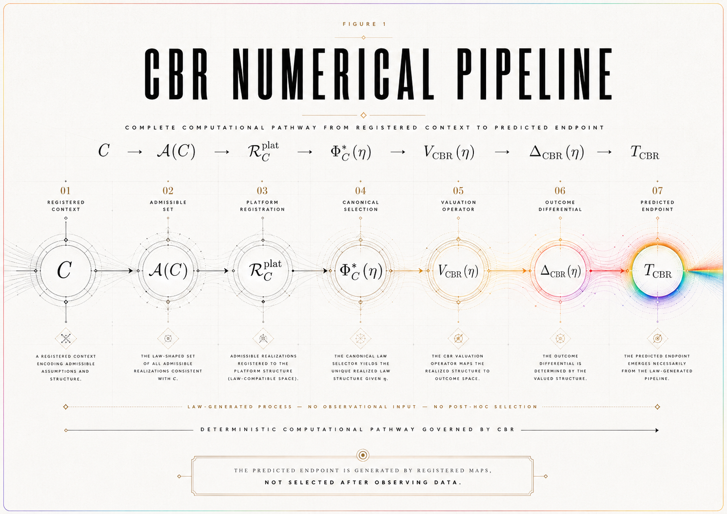
Figure 2 — Candidate-Generation Filters for 𝒜(C)

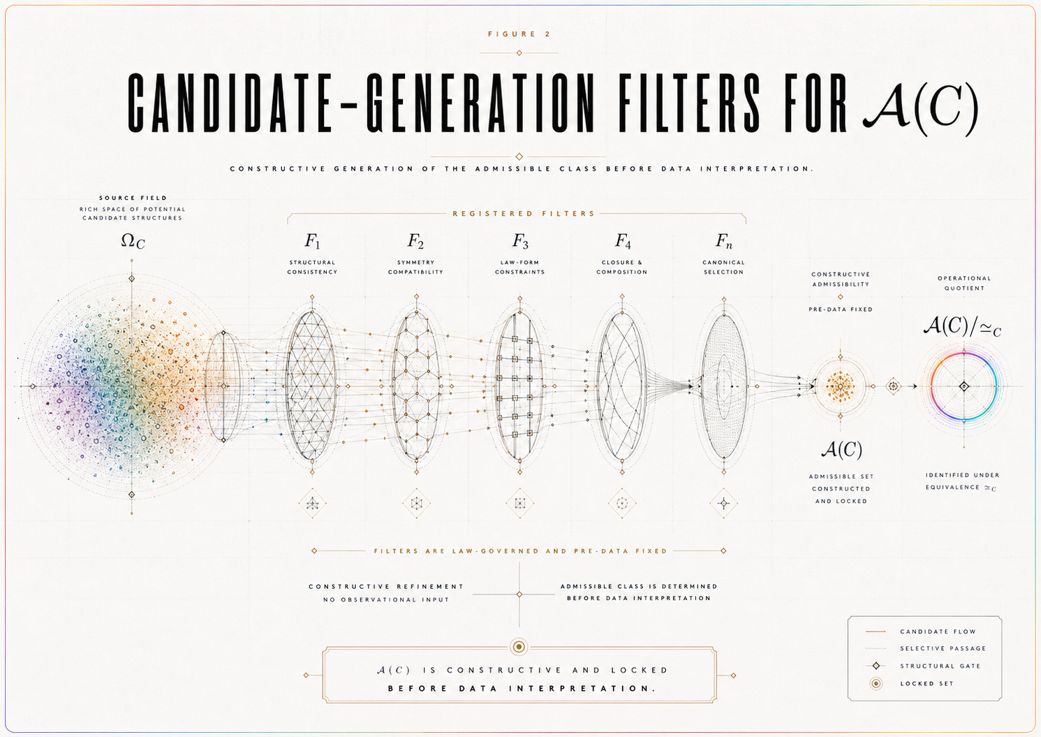
Figure 3 — Burden Proxy Terms Ξ_C, Ω_C, Λ_C

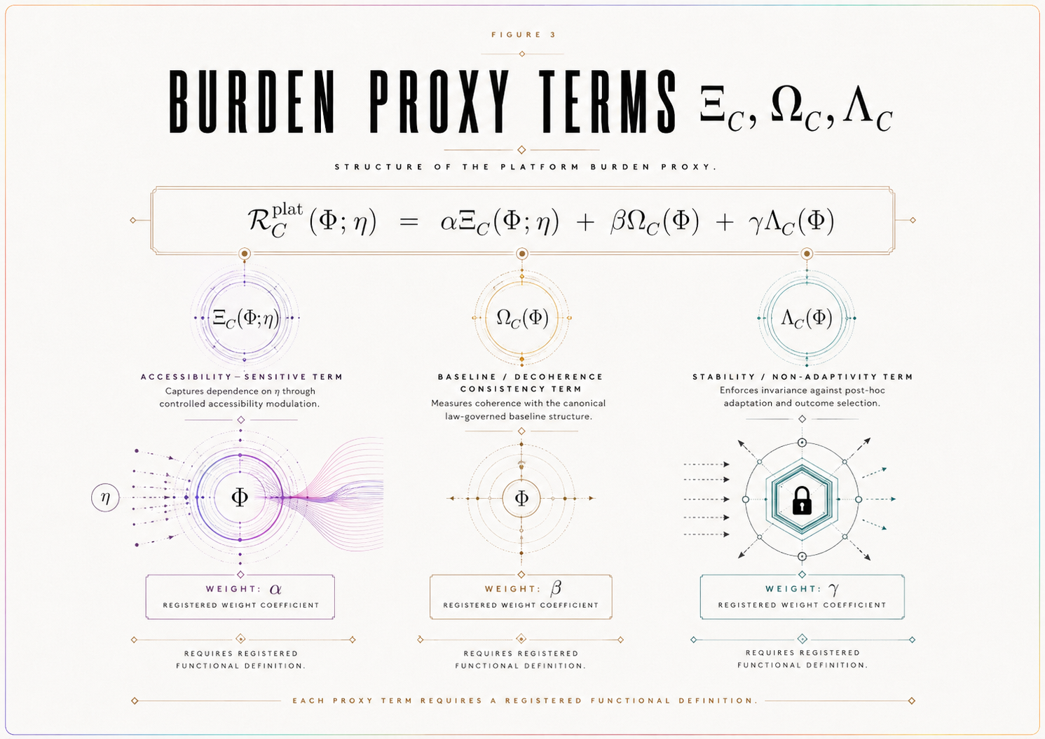
Figure 4 — η Axis with Critical Accessibility Regime I_c

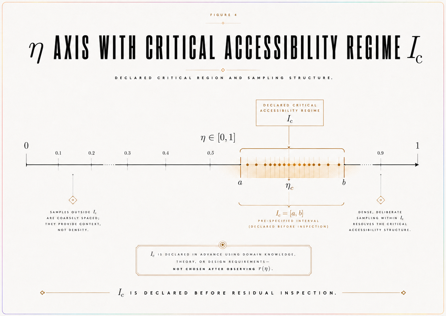
Figure 5 — Baseline Model Class 𝔅 and V_ℬ(η)

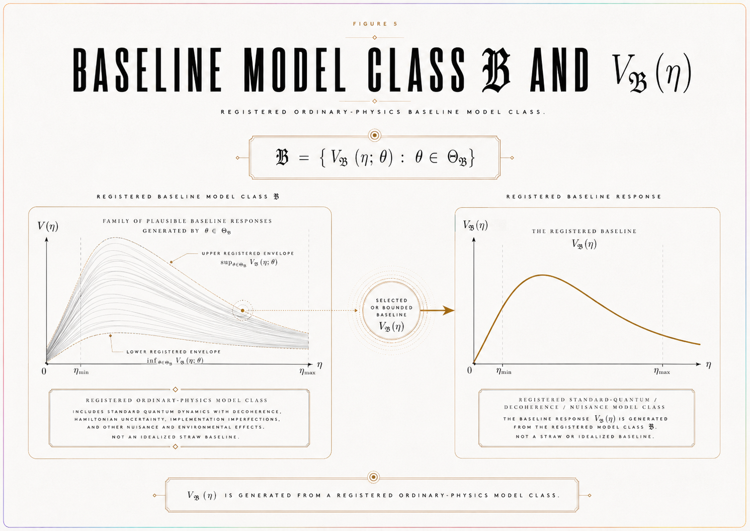
Figure 6 — Nuisance Envelope B_𝓝(η) and Critical Bound B_c

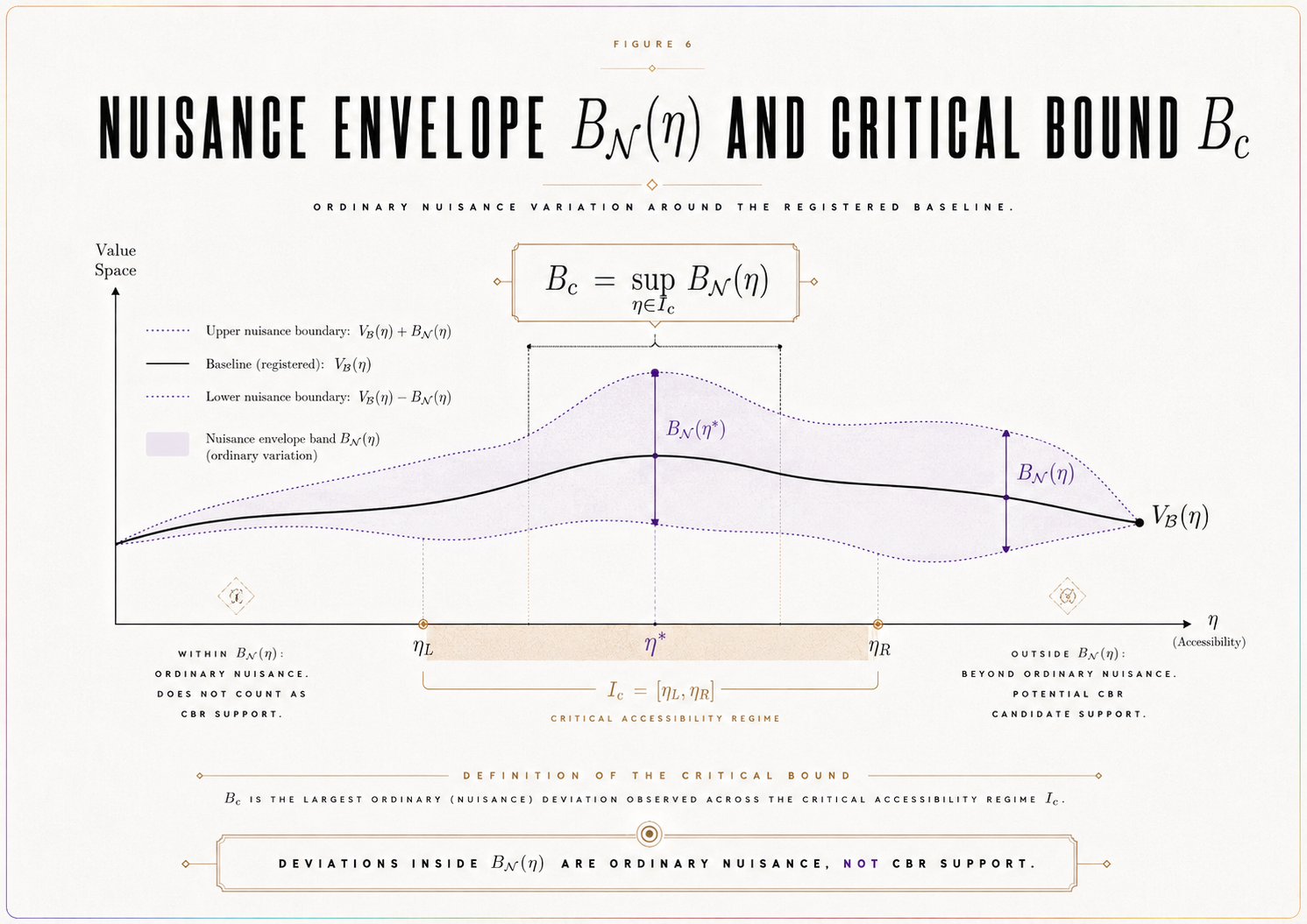
Figure 7 — Decision Threshold Θ_c

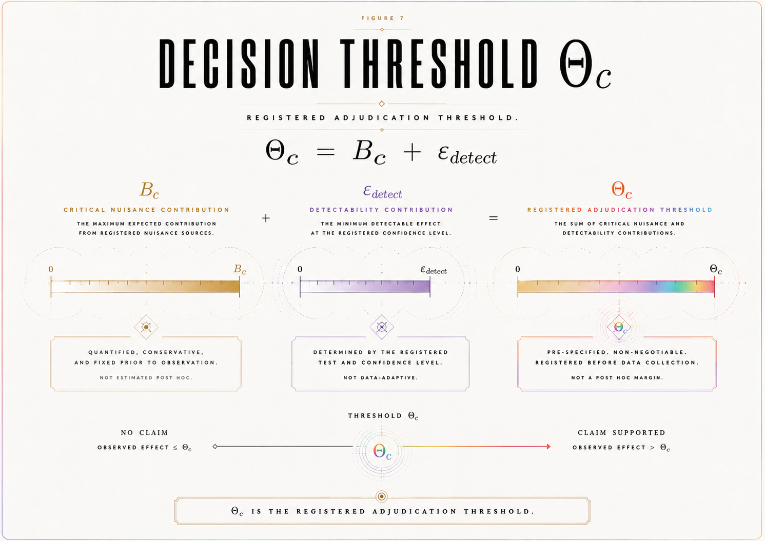
Figure 8 — Example Δ_CBR(η) Morphology

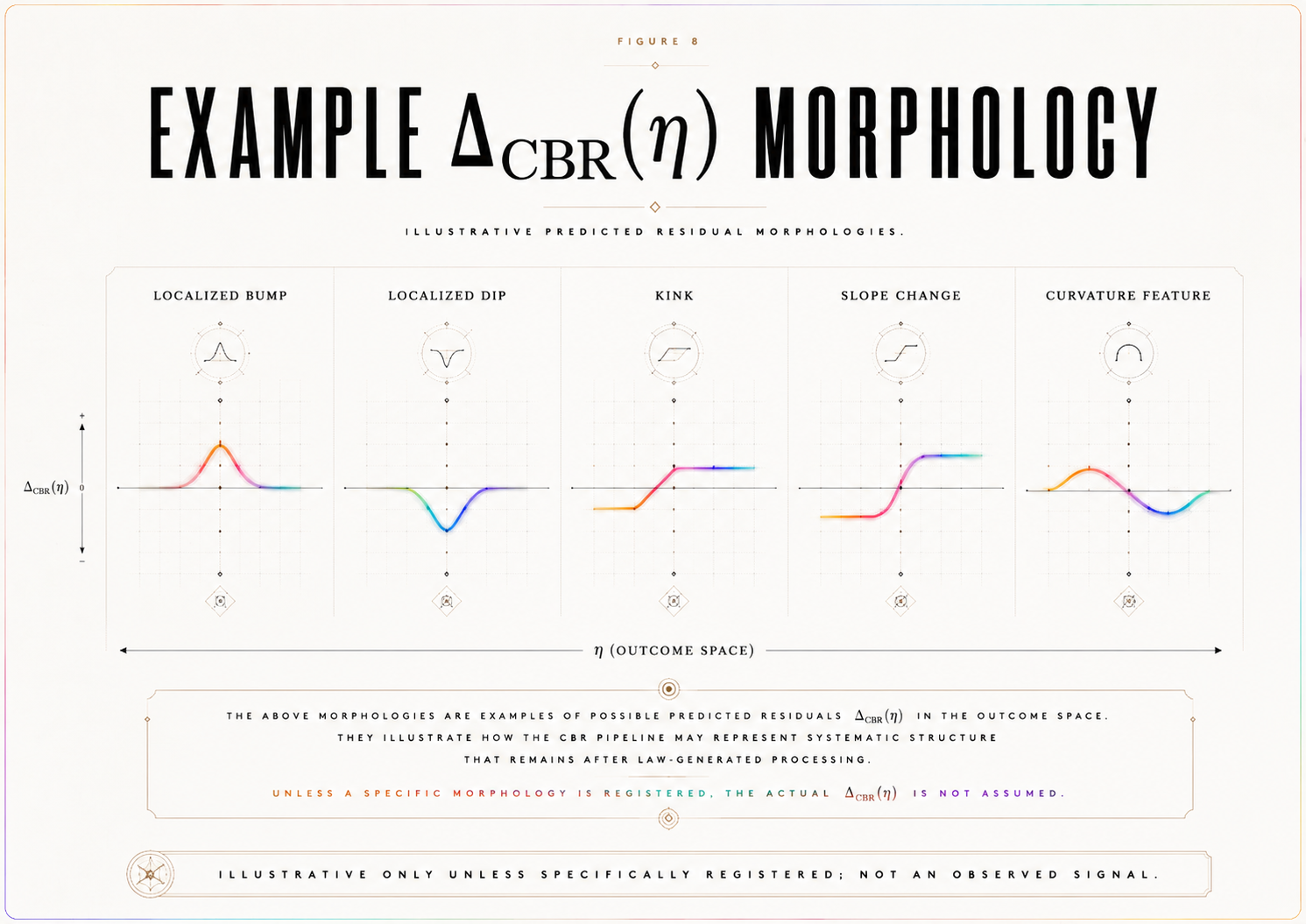
Figure 9 — Endpoint Congruence Between T_c and T_CBR

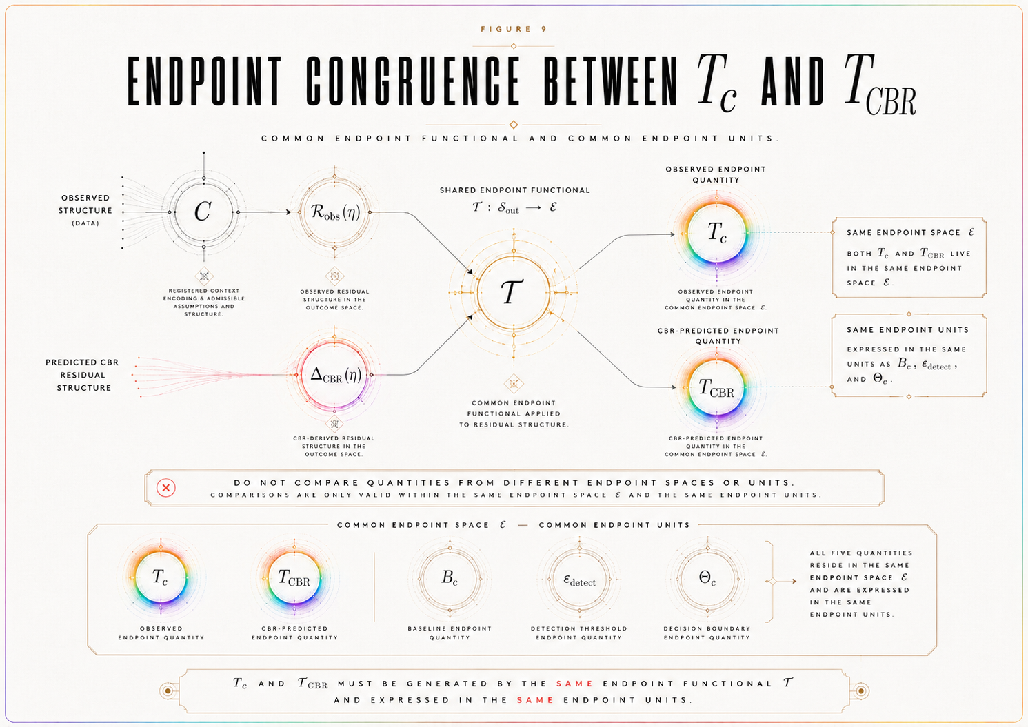
Figure 10 — Identifiability Map

Figure 11 — Verdict Decision Procedure

---

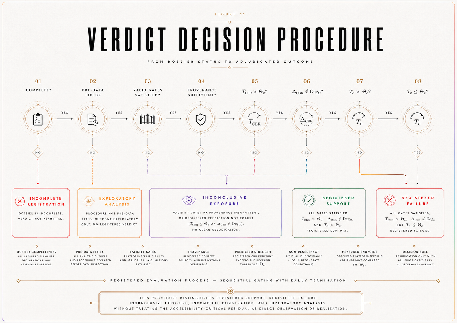
Appendix A — Simulation-Ready Locked Dossier v0.1

A.1 Purpose and Status of This Dossier

This appendix provides the first platform-specific locked dossier for a numerical CBR instantiation in a record-accessibility interferometric context.

Its purpose is not to claim empirical confirmation, registered support, or registered failure. Its purpose is to define the objects required for a simulation-ready CBR platform model and to state which objects are already specified, which are structurally defined, and which remain pending before empirical adjudication could occur.

This dossier version is therefore:

simulation-ready in structure,
not yet adjudication-ready in empirical status.

It prepares the model for simulation, sensitivity analysis, degeneracy testing, and later public-data or experimental comparison. It does not by itself establish that CBR is true, that realization has been observed, or that ordinary quantum/decoherence physics has failed.

A.2 Dossier Identification

Dossier title: Simulation-Ready Locked Dossier for a Platform-Specific Numerical Instantiation of CBR

Dossier short name: CBR-RAI Numerical Dossier

Declared platform: Record-accessibility interferometric context

Dossier version: v0.1

Registration status: Simulation-ready structural dossier; not empirically adjudicative.

Data status:
No observed dataset is used in this dossier version.

Adjudication status:
No registered empirical support or registered empirical failure can be claimed from this version.

Permitted uses:
simulation design, numerical illustration, sensitivity analysis, degeneracy analysis, test-design planning, and preparation for public-data reanalysis.

Not permitted uses:
empirical confirmation, empirical failure, direct observation of realization, or decisive public-data adjudication.

A.3 Audit-Lock Statement

This dossier version fixes the following primary objects at the structural level:

C_RAI,
Ω_C,
𝒜(C_RAI),
≃_C,
ℛ_C^plat,
η,
I_c,
𝔅,
V_ℬ(η),
B_𝓝(η),
B_c,
ε_detect,
Θ_c,
𝒯,
T_c,
T_CBR,
Δ_CBR(η),
Deg_C,
A_stat,
validity gates,
provenance labels,
and verdict categories.

Any change to these objects after data inspection creates a new dossier version. Such a change may define a revised model, but it cannot alter the status of this version.

A.4 No-Adjudication Rule for v0.1

This dossier version is not yet capable of registered empirical support or registered empirical failure.

A registered support or failure verdict requires, at minimum:

fully specified Ξ_C, Ω_C, and Λ_C,
fixed coefficient rules for α, β, and γ,
a calibrated or otherwise justified η,
a platform-justified I_c,
a validated baseline parameter space Θ_ℬ,
a computed nuisance envelope B_𝓝(η),
a computed B_c,
a justified ε_detect,
a fully specified Deg_C,
a fully implemented A_stat,
and either simulated or empirical V_obs(η) sufficient to compute T_c.

Until those objects are completed under registered provenance, this dossier remains simulation-ready but not adjudication-ready.

A.5 Dossier Completion Status

The dossier objects fall into three categories.

A.5.1 Complete at v0.1

The following objects are specified at a usable structural level:

C_RAI — declared platform context.
Ω_C — preliminary candidate space.
𝒜(C_RAI) — admissibility-filter structure.
≃_C — operational-equivalence rule.
η ∈ [0,1] — normalized accessibility range.
I_c = [η_c − w_c, η_c + w_c] ∩ [0,1] — critical-regime form.
𝔅 = {V_ℬ(η; θ) : θ ∈ Θ_ℬ} — baseline-class form.
𝒯_sup — primary endpoint functional.
Δ_CBR(η) = A_CBR g_c(η; η_c, w_r, s) — registered simulation morphology form.
T_CBR = 𝒯_sup[Δ_CBR(η), η ∈ I_c] — predicted endpoint rule.
T_c = 𝒯_sup[V_obs(η) − V_ℬ(η), η ∈ I_c] — observed endpoint rule.
Verdict categories — support, failure, inconclusive, incomplete, exploratory.

A.5.2 Structurally Defined but Pending Functional Completion

The following objects are named and structurally located, but require further functional completion in later appendices:

ℛ_C^plat,
Ξ_C,
Ω_C,
Λ_C,
coefficient rules for α, β, and γ,
normalization conventions,
baseline parameter space Θ_ℬ,
nuisance-combination rule,
detectability calculation,
degeneracy operator Deg_C,
statistical rule A_stat,
and exact validity-gate thresholds.

These objects are not optional. They must be completed before the dossier can become adjudicative.

A.5.3 Required for Empirical Adjudication

The following are required before any empirical verdict can be claimed:

calibrated η,
platform-justified I_c,
validated 𝔅,
selected or fitted V_ℬ(η) under registered rules,
measured, published, calibrated, or derived nuisance terms,
computed B_𝓝(η),
computed B_c,
justified ε_detect,
computed Θ_c,
observed or reconstructable V_obs(η),
computed T_c,
completed Deg_C,
implemented A_stat,
and provenance labels sufficient for the claimed verdict.

A.6 Declared Measurement Context C_RAI

Let C_RAI denote a record-accessibility interferometric context.

The platform is a two-alternative interferometric measurement context in which an interference visibility observable is evaluated while the accessibility of outcome-defining which-path record information is varied.

The context is intended to model delayed-choice, quantum eraser, which-path marking, wave-particle duality, or related interferometric settings at the level required for numerical simulation.

A.6.1 Registered Context Objects

C_RAI includes:

state preparation,
two interferometric alternatives,
which-path or record channel,
record-accessibility control,
visibility readout,
detectors,
phase-control parameters,
possible coincidence or timing windows,
visibility estimator,
η calibration rule,
data-inclusion rule,
validity gates,
and statistical adjudication rule.

A.6.2 Context Limitation

This dossier does not claim to represent all quantum measurements.

It applies only to a record-accessibility interferometric context in which:

η can be operationally defined,
V_obs(η) can be measured or simulated,
V_ℬ(η) can be modeled under ordinary quantum/decoherence/nuisance conditions,
and an accessibility-critical residual can be defined relative to a declared critical regime.

A.7 Preliminary Candidate Space Ω_C

Let Ω_C denote the preliminary platform candidate space.

For this dossier:

Ω_C is the set of platform-compatible candidate maps Φ that assign, for each admissible value of η, a possible visibility-response function:

V_Φ(η)

within the declared context C_RAI.

A candidate Φ ∈ Ω_C is not yet admissible. It becomes admissible only if it passes the registered filters defining 𝒜(C_RAI).

For simulation readiness, candidates may be represented by visibility-response maps of the form:

V_Φ(η) = V_ℬ(η) + Δ_Φ(η),

where Δ_Φ(η) is a candidate residual structure.

The CBR-predicted candidate is the candidate whose residual becomes Δ_CBR(η) after selection by the platform burden proxy.

Provenance status:
model-defined and simulation-ready, not empirically confirmed.

A.8 Admissible Candidate Class 𝒜(C_RAI)

The admissible candidate class is:

𝒜(C_RAI) = {Φ ∈ Ω_C : F_i(Φ, C_RAI) = 1 for all registered filters F_i}.

A candidate enters 𝒜(C_RAI) only if it satisfies all registered admissibility filters.

A.8.1 Registered Filters

A candidate Φ is admissible only if it satisfies the following filters.

F₁ — Context compatibility.
Φ must be defined within C_RAI.

F₂ — Instrument compatibility.
Φ must preserve the registered preparation, interferometric alternatives, record channel, visibility readout, and detector structure.

F₃ — Record-structure compatibility.
Φ must specify how outcome-defining record information is represented as record-accessibility varies.

F₄ — Visibility-response definability.
Φ must generate or determine V_Φ(η).

F₅ — Burden evaluability.
Φ must be evaluable by ℛ_C^plat(Φ; η).

F₆ — Endpoint evaluability.
Φ must allow computation of:

𝒯[V_Φ(η) − V_ℬ(η), η ∈ I_c].

F₇ — Born-discipline constraint.
Φ must not arbitrarily violate ensemble-level quantum statistical structure unless a scoped deviation is explicitly registered.

F₈ — Decoherence/baseline compatibility.
Φ must respect the registered ordinary baseline class 𝔅 except where a CBR residual is explicitly predicted and tested.

F₉ — Non-post-hoc definability.
Φ must be defined before data interpretation.

A.8.2 Status

𝒜(C_RAI) is constructively defined at the filter level.

Detailed mathematical forms for each filter belong in Appendix B.

A.9 Operational Equivalence ≃_C

For Φ₁, Φ₂ ∈ 𝒜(C_RAI):

Φ₁ ≃_C Φ₂

if Φ₁ and Φ₂ are indistinguishable under the registered observables, endpoint functional 𝒯, endpoint-unit convention, uncertainty convention, and statistical rule.

For the primary endpoint used in this dossier:

Φ₁ ≃_C Φ₂

if their endpoint values are statistically indistinguishable:

𝒯[V_Φ₁(η) − V_ℬ(η), η ∈ I_c] ≃ 𝒯[V_Φ₂(η) − V_ℬ(η), η ∈ I_c]

under the registered statistical rule.

If morphology is registered, equivalence also requires morphology-equivalence under the registered morphology comparison.

The actual selection domain is:

𝒜(C_RAI)/≃_C.

A.10 Platform Burden Proxy ℛ_C^plat

This dossier uses a platform-specific burden proxy:

ℛ_C^plat(Φ; η) = αΞ_C(Φ; η) + βΩ_C(Φ) + γΛ_C(Φ).

This is not claimed to be the final universal ℛ_C. It is a registered numerical proxy for the declared platform C_RAI.

A.10.1 Term Roles

Ξ_C(Φ; η) is the accessibility burden term.
It measures how the candidate’s burden varies with record-accessibility.

Ω_C(Φ) is the baseline/decoherence consistency term.
It penalizes candidates that depart from ordinary quantum/decoherence structure except through a registered residual endpoint.

Λ_C(Φ) is the stability/non-adaptivity term.
It penalizes excessive flexibility, post hoc adjustability, or unstable parameterization.

A.10.2 Coefficient Rule

The coefficients α, β, and γ must be fixed before data interpretation.

For this dossier version:

α, β, and γ are symbolic or simulation parameters unless later assigned calibrated, published, derived, or measured values.

They may not be tuned after observing V_obs(η), r(η), T_c, or any simulation outcome intended to imitate empirical adjudication.

A.10.3 Selection Rule

The selected platform candidate is:

Φ∗C(η) ∈ argmin{Φ ∈ 𝒜(C_RAI)} ℛ_C^plat(Φ; η), up to ≃_C.

This selection rule is defined at the platform-proxy level.

A.10.4 Status

ℛ_C^plat is registered structurally in this dossier.

The detailed functional definitions of Ξ_C, Ω_C, Λ_C, normalization, coefficient domains, and data-independence conditions must be supplied in Appendix C.

Until those details are filled, the model is not adjudication-ready.

A.11 Record-Accessibility Variable η

Let η denote operational record-accessibility.

For C_RAI, η is a normalized accessibility variable measuring the degree to which outcome-defining which-path record information is accessible in the platform.

η is not consciousness.
η is not subjective awareness.
η is not metaphysical observation.
η is not human knowledge.

It is an operational accessibility parameter.

A.11.1 Range

For the first numerical instantiation:

η ∈ [0,1].

Interpretation:

η = 0 means no accessible outcome-defining which-path record under the registered accessibility proxy.

η = 1 means maximal accessible outcome-defining which-path record under the registered accessibility proxy.

A.11.2 Candidate Platform Proxies

Acceptable operational proxies may include:

which-path distinguishability,
record-retention probability,
marker strength,
eraser accessibility,
path-knowledge parameter,
coincidence-conditioned accessibility,
or another registered platform-specific accessibility estimator.

A.11.3 Calibration Status

For this dossier version, η calibration is required for future testing unless a specific dataset or platform supplies a validated calibration rule.

For simulation, η may be sampled over a registered grid:

η_j ∈ [0,1]

with grid spacing Δη labeled simulated or illustrative.

A.12 Critical Accessibility Regime I_c

The critical accessibility regime is the region in which the registered CBR endpoint is predicted to be most identifiable.

For the simulation-ready model, define:

I_c = [η_c − w_c, η_c + w_c] ∩ [0,1].

A simple illustrative center is:

η_c = 1/2

with width:

w_c > 0

fixed before endpoint evaluation.

A.12.1 Provenance

In this dossier version:

η_c is illustrative or model-registered.
w_c is illustrative or model-registered.
I_c is simulation-ready, not empirically calibrated.

For empirical adjudication, η_c and I_c must be justified by a platform-specific bridge, calibration model, or prior registered theoretical commitment.

A.12.2 Lock Rule

I_c may not be chosen after inspecting r(η).

Changing I_c after residual inspection creates a new dossier version.

A.13 Baseline Model Class 𝔅

Let:

𝔅 = {V_ℬ(η; θ) : θ ∈ Θ_ℬ}.

Here Θ_ℬ is the ordinary-physics parameter space for the declared platform.

A.13.1 Baseline Family

For the first numerical instantiation, the baseline family should include ordinary visibility reduction associated with record-accessibility, plus platform nuisance and decoherence effects.

A simulation-ready schematic family is:

V_ℬ(η; θ) = V₀ f_Q(η; q) D_decoh(η; κ) + d(η; λ),

where:

V₀ is nominal visibility scale,
f_Q(η; q) is the ordinary quantum/interferometric visibility-accessibility response,
D_decoh(η; κ) is an ordinary decoherence or loss factor,
d(η; λ) is a registered drift or calibration component allowed by the baseline class,
and θ = (V₀, q, κ, λ).

A.13.2 Example Baseline Component

For simulation only, one may use:

f_Q(η; q) = (1 − η^q)^{1/q}

with q ≥ 1.

A simpler illustrative model may set:

f_Q(η) = √(1 − η²).

These are illustrative ordinary visibility-accessibility responses, not empirical claims unless calibrated, derived, measured, or published under valid rules.

The chosen form must be registered before simulation or data comparison.

A.13.3 Included Ordinary Effects

The baseline class must include, where applicable:

standard quantum visibility behavior,
decoherence,
detector inefficiency,
dark counts,
loss,
phase drift,
finite sampling,
calibration uncertainty,
alignment uncertainty,
visibility-estimator uncertainty,
environmental noise,
postselection effects,
and timing or coincidence-window effects.

A.13.4 Baseline Status

For this dossier version, 𝔅 is symbolic or simulation-ready.

For empirical adjudication, Θ_ℬ, V₀, q, κ, λ, and any drift parameters must be measured, published, calibrated, or derived under registered rules.

A.14 Selected Baseline Visibility V_ℬ(η)

The selected baseline visibility curve is:

V_ℬ(η) = V_ℬ(η; θ₀),

where θ₀ ∈ Θ_ℬ is selected by the registered baseline-selection rule.

A.14.1 Selection Rule

In this dossier version, θ₀ may be:

symbolic for analytic work,
illustrative for exposition,
simulated for the simulation paper,
published if drawn from existing platform literature,
calibrated if a platform calibration is provided,
or measured if derived from actual test data under locked rules.

A.14.2 Anti-Overfitting Rule

θ₀ cannot be refit after inspecting r(η) in a way that changes the verdict.

A new θ₀ selected after residual inspection creates a new dossier version.

A.15 Nuisance Envelope B_𝓝(η)

Let B_𝓝(η) denote the registered nuisance envelope around V_ℬ(η).

A simulation-ready form is:

B_𝓝(η) = [σ_det²(η) + σ_phase²(η) + σ_cal²(η) + σ_sample²(η) + σ_η²(η)|∂_η V_ℬ(η)|² + σ_est²(η)]^{1/2}.

This expression treats nuisance contributions in quadrature.

A.15.1 Included Sources

The envelope includes:

detector noise,
phase instability,
calibration uncertainty,
finite sampling,
η uncertainty propagated through V_ℬ(η),
visibility-estimator uncertainty,
background-count uncertainty,
alignment uncertainty,
and platform drift.

A.15.2 Provenance

In this dossier version, the nuisance components are symbolic or simulation-ready.

For empirical adjudication, each term must be measured, published, calibrated, or derived.

A.15.3 Lock Rule

B_𝓝(η) cannot be widened after inspecting r(η).

A.16 Critical Nuisance Bound B_c

For a supremum endpoint:

B_c = sup_{η ∈ I_c} B_𝓝(η).

If the endpoint is normalized, integrated, morphology-sensitive, or model-comparison based, B_c must be transformed into the same endpoint units as T_c and T_CBR.

For this dossier version, B_c is symbolic or simulation-ready.

For adjudication, B_c must be computed from registered nuisance quantities.

A.17 Detectability Threshold ε_detect

Let ε_detect denote the minimum endpoint separation required for the platform to distinguish a residual from baseline-plus-nuisance behavior.

For the simulation-ready supremum endpoint, a symbolic form is:

ε_detect = z_detect σ_T,

where:

z_detect is the registered sensitivity or confidence multiplier,
and σ_T is the endpoint-level uncertainty scale.

A.17.1 Provenance

In this dossier version:

z_detect is an assumed or simulation parameter.
σ_T is derived from symbolic nuisance and sampling terms.
ε_detect is simulation-ready, not empirically measured.

For empirical adjudication, ε_detect must be justified by platform sensitivity, power analysis, sampling density, visibility resolution, and statistical rule.

A.18 Decision Threshold Θ_c

The registered decision threshold is:

Θ_c = B_c + ε_detect.

A.18.1 Role

Support requires:

T_c > Θ_c

under valid conditions and with registered morphology satisfied.

Failure requires:

T_CBR > Θ_c

and:

T_c ≤ Θ_c

under valid conditions, with Δ_CBR ∉ Deg_C.

A.18.2 Status

For this dossier version, Θ_c is symbolic or simulation-ready.

A.19 Endpoint Functional 𝒯

For the first numerical instantiation, use the primary endpoint functional:

𝒯_sup[x(η), η ∈ I_c] = sup_{η ∈ I_c} |x(η)|.

Thus:

T_c = sup_{η ∈ I_c} |V_obs(η) − V_ℬ(η)|

and:

T_CBR = sup_{η ∈ I_c} |Δ_CBR(η)|.

A.19.1 Endpoint Units

The endpoint units are visibility units.

Therefore:

B_c,
ε_detect,
Θ_c,
T_c,
and T_CBR

must all be expressed in visibility units.

A.19.2 Secondary Endpoints

Secondary endpoints may be used for diagnostics only.

They do not control the decisive verdict in this dossier version.

A.20 Predicted Residual Δ_CBR(η)

The predicted CBR residual is:

Δ_CBR(η) = V_CBR(η) − V_ℬ(η).

For simulation readiness, register a localized accessibility-critical morphology:

Δ_CBR(η) = A_CBR g_c(η; η_c, w_r, s),

where:

A_CBR is the predicted residual amplitude,
g_c is a normalized localized shape function,
η_c is the critical accessibility center,
w_r is residual width,
and s ∈ {+1, −1} determines residual sign.

A simple registered morphology is:

g_c(η; η_c, w_r, s) = s exp[−(η − η_c)²/(2w_r²)].

A.20.1 Provenance

For this dossier version:

A_CBR is an assumed or simulation parameter unless derived from a completed ℛ_C^plat computation.
η_c is illustrative or model-registered.
w_r is illustrative or simulation parameter.
s is a registered model choice.

This residual is not empirical evidence. It is the model’s simulation-ready predicted morphology.

A.20.2 Endpoint Prediction

For the supremum endpoint:

T_CBR = sup_{η ∈ I_c} |A_CBR g_c(η; η_c, w_r, s)|.

If η_c ∈ I_c and g_c is normalized to unit maximum, then:

T_CBR = |A_CBR|.

This equality is valid only under the registered morphology and endpoint convention.

A.21 CBR-Predicted Visibility V_CBR(η)

The predicted CBR-side visibility response is:

V_CBR(η) = V_ℬ(η) + Δ_CBR(η).

Equivalently:

V_CBR(η) = V_ℬ(η) + A_CBR g_c(η; η_c, w_r, s).

This is a simulation-ready model response, not an observed curve.

The observed curve, if available later, is V_obs(η).

A.22 Observed Endpoint T_c

If observed or simulated data are available:

T_c = sup_{η ∈ I_c} |V_obs(η) − V_ℬ(η)|.

In simulation, V_obs(η) may be generated under:

baseline-only conditions,
CBR-positive conditions,
strong-null conditions,
wide-nuisance conditions,
underpowered conditions,
η-miscalibration conditions,
or degeneracy conditions.

For this dossier version, T_c is not yet empirical because no observed dataset is supplied.

A.23 Degeneracy Operator Deg_C

Let Deg_C denote the ordinary-degeneracy class for the declared platform.

Δ_CBR ∈ Deg_C if the predicted residual can be absorbed, reproduced, or rendered statistically indistinguishable by registered ordinary transformations.

These transformations include:

baseline parameter shifts θ → θ′ inside Θ_ℬ,
nuisance deformations δ_𝓝(η) bounded by B_𝓝(η),
η calibration perturbations,
phase-drift deformations,
detector-response changes,
postselection or coincidence-window effects,
visibility-estimator bias,
finite-sampling fluctuations,
and endpoint-statistic ambiguity.

A.23.1 Degeneracy Test

The dossier tests whether there exists an allowed ordinary transformation such that:

𝒯[Δ_CBR(η), η ∈ I_c]

is indistinguishable from ordinary baseline-plus-nuisance behavior under the registered statistical rule.

If yes:

Δ_CBR ∈ Deg_C

and the endpoint is non-identifiable.

If no:

Δ_CBR ∉ Deg_C

and the endpoint passes the identifiability condition, provided T_CBR > Θ_c.

A.23.2 Status

For this dossier version, Deg_C is structurally defined.

Appendix H must fill the exact degeneracy transformations and decision rule.

A.24 Statistical Rule A_stat

Let A_stat denote the registered statistical adjudication rule.

For this simulation-ready version, A_stat must determine:

whether T_c > Θ_c,
whether T_c ≤ Θ_c,
whether morphology is satisfied,
whether Δ_CBR ∈ Deg_C,
whether sampling inside I_c is adequate,
and whether uncertainty permits adjudication.

A.24.1 Minimal Rule

A minimal rule is:

support-eligible if T_c > Θ_c under valid conditions and Δ_CBR ∉ Deg_C;

failure-eligible if T_CBR > Θ_c, Δ_CBR ∉ Deg_C, and T_c ≤ Θ_c under valid conditions;

inconclusive if detectability, identifiability, sampling, calibration, baseline, nuisance, or provenance conditions fail.

A.24.2 Status

For this dossier version, A_stat is registered structurally and must be specified numerically in the simulation paper or later empirical test.

A.25 Validity Gates

A test or simulation must satisfy the following validity gates.

η calibration gate:
η is defined, sampled, and uncertainty-bounded.

Critical-regime gate:
I_c is fixed before endpoint computation.

Baseline gate:
𝔅 and V_ℬ(η) are registered and non-adaptive.

Nuisance gate:
B_𝓝(η) and B_c are registered in endpoint units.

Detectability gate:
ε_detect and Θ_c are defined.

Endpoint gate:
𝒯, T_c, and T_CBR use the same endpoint units.

Identifiability gate:
Δ_CBR ∉ Deg_C.

Provenance gate:
The required values have provenance labels sufficient for the claimed verdict.

Statistical gate:
A_stat can adjudicate the comparison.

Failure of any gate prevents registered support or registered failure.

A.26 Parameter Provenance Registry

A.26.1 Current Provenance Labels

C_RAI: model-defined / declared platform.
Ω_C: model-defined.
𝒜(C_RAI): generated by registered filters; detailed filters required.
≃_C: registered operational relation.
ℛ_C^plat: structurally defined; detailed functional terms required.
α, β, γ: symbolic / simulation parameters unless later fixed.
η: operational variable; calibration required for empirical adjudication.
I_c: illustrative / simulation-ready unless platform-justified.
𝔅: symbolic / simulation-ready baseline class.
V_ℬ(η): symbolic or simulated unless calibrated/published.
B_𝓝(η): symbolic / simulation-ready.
B_c: derived symbolically from B_𝓝(η).
ε_detect: symbolic / simulation parameter.
Θ_c: derived symbolically from B_c + ε_detect.
𝒯: registered endpoint functional.
Δ_CBR(η): assumed / simulation morphology unless derived from completed burden proxy.
T_CBR: derived from Δ_CBR(η) under 𝒯.
T_c: unavailable until simulation or data.
Deg_C: structurally defined; detailed transformations required.
A_stat: structurally registered; numerical implementation required.

A.26.2 Provenance-Limited Status

This dossier version can support:

numerical illustration,
simulation readiness,
test-design planning,
and conditional analysis.

It cannot support:

empirical confirmation,
empirical failure,
or decisive public-data adjudication.

A.27 Verdict Rules

A.27.1 Registered Support

Registered support requires:

T_c > Θ_c,
registered morphology satisfied where applicable,
Δ_CBR ∉ Deg_C,
baseline separation,
nuisance separation,
η calibration valid,
data adequate,
provenance sufficient,
validity gates passed,
and A_stat satisfied.

This dossier version cannot yet claim registered empirical support because T_c is not supplied by observed data.

A.27.2 Registered Failure

Registered failure requires:

T_CBR > Θ_c,
Δ_CBR ∉ Deg_C,
valid test conditions,
and:

T_c ≤ Θ_c.

This dossier version cannot yet claim registered empirical failure because no observed T_c is supplied.

A.27.3 Inconclusive Exposure

The result is inconclusive if the model is registered but calibration, baseline, nuisance, detectability, sampling, identifiability, provenance, or statistical conditions are insufficient.

A.27.4 Incomplete Registration

The dossier is incomplete for empirical adjudication until the following are fully specified:

functional forms for Ξ_C, Ω_C, Λ_C,
coefficient rules for α, β, γ,
calibrated or justified η,
specific I_c,
validated 𝔅,
computed B_𝓝(η) and B_c,
empirical or simulated ε_detect,
fully specified Deg_C,
and implemented A_stat.

A.27.5 Exploratory Status

If any primary object is selected after inspecting data, the analysis is exploratory.

A.28 Simulation Export File

This dossier exports the following objects to the simulation paper.

Platform:C_RAI.
η range:η ∈ [0,1].
η grid: to be selected before simulation.
Critical regime:I_c = [η_c − w_c, η_c + w_c] ∩ [0,1].
Baseline class:𝔅 = {V_ℬ(η; θ) : θ ∈ Θ_ℬ}.
Baseline curve:V_ℬ(η; θ₀).
Nuisance envelope:B_𝓝(η).
Critical nuisance bound:B_c = sup_{η ∈ I_c} B_𝓝(η).
Detectability threshold:ε_detect = z_detect σ_T.
Decision threshold:Θ_c = B_c + ε_detect.
Residual morphology:Δ_CBR(η) = A_CBR g_c(η; η_c, w_r, s).
Endpoint functional:𝒯_sup.
Predicted endpoint:T_CBR = sup_{η ∈ I_c} |Δ_CBR(η)|.
Observed endpoint rule:T_c = sup_{η ∈ I_c} |V_obs(η) − V_ℬ(η)|.
Degeneracy operator:Deg_C, structurally defined.
Statistical rule:A_stat, structurally defined.
Validity gates: listed in A.25.
Provenance labels: listed in A.26.

The simulation paper must not invent new primary objects. If it does, it defines a new dossier version.

A.29 Final Dossier Status

This Appendix A fills the platform dossier at a simulation-ready structural level.

It establishes:

a declared platform context,
a candidate-space structure,
an admissible candidate-generation rule,
a platform burden-proxy structure,
an operational η variable,
a critical accessibility regime,
a baseline model class,
a nuisance envelope form,
a decision threshold,
a primary endpoint functional,
a predicted residual morphology,
a predicted endpoint rule,
a degeneracy operator,
a statistical-rule placeholder,
validity gates,
provenance labels,
verdict rules,
and simulation-export objects.

It does not establish empirical support or failure.

Its strongest legitimate status is:

simulation-ready numerical instantiation, pending full functional specification of ℛ_C^plat, Deg_C, A_stat, and platform-calibrated parameter values.

Appendix B — Candidate-Generation Filters

B.1 Purpose of Appendix B

This appendix defines the admissibility filters used to generate the platform-specific candidate class 𝒜(C_RAI) from the preliminary candidate space Ω_C.

The purpose is to make 𝒜(C_RAI) constructive, auditable, and non-post-hoc. A candidate is not admissible merely because it can be written down, fitted to data, or interpreted after the fact. A candidate is admissible only if it passes the registered filters below before endpoint evaluation.

This appendix supports the construction rule:

𝒜(C_RAI) = {Φ ∈ Ω_C : F_i(Φ, C_RAI) = 1 for all registered filters F_i}.

The filters do not prove CBR. They define the platform-specific domain over which the burden proxy ℛ_C^plat may operate.

The hierarchy remains:

The law is constrained selection.
The residual is the fingerprint.
The strong null is the wound.

Candidate admissibility is therefore not empirical support. It is the precondition for lawful evaluation.

B.2 Declared Candidate Space Ω_C

Let Ω_C denote the preliminary candidate space for the declared record-accessibility interferometric context C_RAI.

For this numerical instantiation, a preliminary candidate Φ ∈ Ω_C is a platform-compatible candidate response model containing, at minimum:

V_Φ(η) — a candidate visibility-response function;
Δ_Φ(η) — the candidate residual relative to the registered baseline, where applicable;
M_Φ — a morphology descriptor if the candidate predicts localized structure;
P_Φ — candidate parameters or internal model commitments;
S_Φ — provenance status indicating whether the candidate is symbolic, illustrative, simulated, assumed, derived, calibrated, published, measured, or required for future testing.

A candidate becomes admissible only if it passes every registered filter F_i.

The admissible class is therefore:

𝒜(C_RAI) ⊂ Ω_C.

The quotient class used for selection is:

𝒜(C_RAI)/≃_C.

B.3 Canonical Candidate Families

The preliminary candidate space Ω_C may contain several candidate families. These families are listed to make the space less abstract and to clarify which candidates are admissible, non-admissible, identifiable, or non-identifiable.

B.3.1 Baseline-Equivalent Candidates

Baseline-equivalent candidates satisfy:

Δ_Φ(η) = 0

or generate residuals fully absorbed by the registered baseline model class 𝔅.

These candidates may be admissible if they pass the filters, but they do not provide CBR support because they do not generate an accessibility-critical residual.

B.3.2 Nuisance-Degenerate Candidates

Nuisance-degenerate candidates generate residuals satisfying:

Δ_Φ ∈ Deg_C

or residuals lying within the registered nuisance envelope B_𝓝(η).

Such candidates may be admissible for evaluation, but they are not identifiable as CBR-supporting endpoints.

B.3.3 Accessibility-Sensitive CBR Candidates

Accessibility-sensitive candidates contain nontrivial dependence on η through the registered burden proxy ℛ_C^plat and generate a candidate residual Δ_Φ(η) that can be evaluated by the endpoint functional 𝒯.

These are the primary candidates relevant to CBR endpoint testing.

B.3.4 Born-Disciplined Candidates

Born-disciplined candidates preserve ensemble-level quantum statistical structure or register a scoped and explicit deviation with its own endpoint and failure rule.

These candidates pass the probability-discipline requirement only if they avoid arbitrary outcome-weight engineering.

B.3.5 Born-Violating Candidates

Born-violating candidates introduce unregistered probability distortions, arbitrary weighting, or post hoc ensemble adjustments.

These candidates are excluded unless the deviation is explicitly registered as part of the dossier with its own baseline, endpoint, and failure rule.

B.3.6 Post Hoc Candidates

Post hoc candidates are introduced, reshaped, or reparameterized after inspecting V_obs(η), r(η), T_c, or the verdict.

These candidates are excluded from the registered dossier. They may motivate a future dossier version, but they cannot support or rescue the present one.

B.4 Filter Output Convention

Each filter F_i is a binary admissibility rule:

F_i(Φ, C_RAI) ∈ {0,1}.

The convention is:

F_i(Φ, C_RAI) = 1 means Φ passes the filter.
F_i(Φ, C_RAI) = 0 means Φ fails the filter.

A candidate is admissible only if:

F₁(Φ, C_RAI) = F₂(Φ, C_RAI) = ⋯ = F₉(Φ, C_RAI) = 1.

Equivalently:

Φ ∈ 𝒜(C_RAI) ⇔ Φ ∈ Ω_C and ∏_{i=1}^{9} F_i(Φ, C_RAI) = 1.

A failed filter excludes the candidate from the registered admissible class for this dossier version.

A candidate excluded by the filters may be studied in a later dossier version, but it is not part of 𝒜(C_RAI) for the present instantiation.

B.5 Principle — Filter Independence

Each admissibility filter F_i must be evaluable without access to V_obs(η), r(η), T_c, or the realized verdict. A filter that depends on the observed residual is not an admissibility filter; it is a post hoc selection rule.

This principle is essential. If the filters depend on the outcome, the admissible class is not fixed before selection. If the admissible class is not fixed before selection, the law-form is not exposed to failure.

Admissibility must therefore be determined from registered platform structure, not from observed residual success.

B.6 Definition — Admissibility Certificate

For every admitted candidate Φ ∈ 𝒜(C_RAI), the dossier must provide an admissibility certificate:

Cert(Φ) = {F₁(Φ), F₂(Φ), …, F₉(Φ), provenance(Φ), endpoint status, burden-evaluability status, equivalence class [Φ]_≃C}.

A candidate is admissible only if:

F_i(Φ) = 1 for all i,
the candidate has a registered provenance label,
the candidate is evaluable by ℛ_C^plat,
the candidate is evaluable by 𝒯,
and the candidate has a defined operational equivalence class under ≃_C.

If a candidate lacks a complete certificate, it is not admissible in this dossier version.

The certificate makes candidate admission auditable rather than discretionary.

B.7 Filter F₁ — Context Compatibility

B.7.1 Role

The context-compatibility filter ensures that a candidate belongs to the declared platform context C_RAI.

A candidate must not silently change the measurement context, platform assumptions, accessibility mechanism, visibility readout, or data-inclusion rule.

B.7.2 Criterion

A candidate Φ passes F₁ only if it is defined within the fixed context C_RAI.

That requires Φ to preserve:

state preparation,
two interferometric alternatives,
record-accessibility structure,
visibility readout,
detector model,
phase-control convention,
data-inclusion rule,
η domain,
critical-regime convention,
and endpoint-statistic convention.

Formally:

F₁(Φ, C_RAI) = 1

only if:

Dom(Φ) ⊆ Dom(C_RAI)

and the response map V_Φ(η) is defined over the registered accessibility domain.

B.7.3 Failure Condition

F₁(Φ, C_RAI) = 0 if Φ requires a different platform context, different measurement basis, different accessibility variable, different visibility estimator, or altered data-inclusion rule.

B.7.4 Lock Rule

The context cannot be changed after data interpretation to admit a candidate that otherwise fails F₁.

Such a change creates a new dossier version.

B.8 Filter F₂ — Instrument Compatibility

B.8.1 Role

The instrument-compatibility filter ensures that candidate behavior is generated within the registered preparation-measurement-readout structure.

A candidate cannot be admissible if it requires an unregistered instrument, hidden detector modification, altered coincidence logic, or unregistered postselection rule.

B.8.2 Criterion

A candidate Φ passes F₂ only if it respects the registered instrument architecture of C_RAI:

preparation map,
interferometric alternatives,
which-path or record channel,
accessibility-control operation,
readout operation,
detector response model,
and timing or coincidence rule where applicable.

If 𝓘_C denotes the registered platform instrument structure, then:

F₂(Φ, C_RAI) = 1

only if Φ is evaluable within 𝓘_C without modifying 𝓘_C.

B.8.3 Failure Condition

F₂(Φ, C_RAI) = 0 if Φ requires an unregistered change to the instrument, detector model, coincidence window, postselection procedure, or visibility readout.

B.8.4 Lock Rule

Instrument parameters may be calibrated under registered rules, but the instrument structure may not be changed after residual inspection to admit or rescue a candidate.

B.9 Filter F₃ — Record-Structure Compatibility

B.9.1 Role

The record-structure filter ensures that a candidate explicitly represents the outcome-defining record structure whose accessibility is varied by η.

Because the platform is a record-accessibility interferometric context, a candidate must specify how record information exists, is marked, erased, retained, degraded, or made accessible within the declared model.

B.9.2 Criterion

A candidate Φ passes F₃ only if it defines a record-structure map:

R_Φ : η ↦ record-accessibility state

or an equivalent registered representation linking η to outcome-defining record information.

The candidate must specify how changes in η affect the record-accessibility status relevant to the platform.

B.9.3 Failure Condition

F₃(Φ, C_RAI) = 0 if Φ treats η as a decorative parameter, subjective observation, human awareness, or post hoc label rather than an operational record-accessibility variable.

It also fails if the candidate gives no account of how record-accessibility enters the platform response.

B.9.4 Lock Rule

The record-structure interpretation of η must be fixed before endpoint evaluation. It may not be reconstructed after seeing V_obs(η) or r(η).

B.10 Filter F₄ — Visibility-Response Definability

B.10.1 Role

The visibility-response filter ensures that every admissible candidate can generate the observable required by the endpoint test.

CBR does not claim to observe realization directly. The platform test requires a visibility-level endpoint. Therefore, each admissible candidate must determine or entail a candidate visibility response.

B.10.2 Criterion

A candidate Φ passes F₄ only if it defines:

V_Φ(η)

over the registered accessibility domain, and if V_Φ(η) can be compared with the baseline curve V_ℬ(η).

The candidate residual is then:

Δ_Φ(η) = V_Φ(η) − V_ℬ(η).

The candidate must also allow endpoint evaluation:

𝒯[Δ_Φ(η), η ∈ I_c].

B.10.3 Failure Condition

F₄(Φ, C_RAI) = 0 if Φ does not determine a visibility response, does not define a residual relative to V_ℬ(η), or cannot be evaluated over I_c.

B.10.4 Lock Rule

The visibility-response rule must be registered before endpoint evaluation. A candidate cannot be admitted by inventing V_Φ(η) after observing the residual curve.

B.11 Filter F₅ — Burden Evaluability

B.11.1 Role

The burden-evaluability filter ensures that every admissible candidate lies within the domain of the platform burden proxy ℛ_C^plat.

The selection rule:

Φ∗C(η) ∈ argmin{Φ ∈ 𝒜(C_RAI)} ℛ_C^plat(Φ; η), up to ≃_C

is meaningless unless ℛ_C^plat(Φ; η) can be evaluated for every Φ ∈ 𝒜(C_RAI).

B.11.2 Criterion

A candidate Φ passes F₅ only if the following quantities are defined for Φ:

Ξ_C(Φ; η),
Ω_C(Φ),
Λ_C(Φ),

and therefore:

ℛ_C^plat(Φ; η) = αΞ_C(Φ; η) + βΩ_C(Φ) + γΛ_C(Φ).

The candidate must be evaluable over the registered η domain and, where relevant, over I_c.

B.11.3 Failure Condition

F₅(Φ, C_RAI) = 0 if any term of ℛ_C^plat is undefined for Φ, if coefficient application is undefined, or if the burden value depends on outcome inspection.

B.11.4 Lock Rule

A candidate cannot be admitted by defining a new burden term after the residual is known. Any such change creates a new dossier version.

B.12 Filter F₆ — Endpoint Evaluability

B.12.1 Role

The endpoint-evaluability filter ensures that every admissible candidate can be assessed by the registered endpoint functional 𝒯.

A candidate may have a visibility response and burden value but still fail endpoint evaluability if it cannot be expressed in the endpoint space used by the test.

B.12.2 Criterion

A candidate Φ passes F₆ only if:

𝒯[V_Φ(η) − V_ℬ(η), η ∈ I_c]

is defined in the same endpoint units as:

B_c,
ε_detect,
Θ_c,
T_c,
and T_CBR.

For the dossier’s primary endpoint:

𝒯_sup[x(η), η ∈ I_c] = sup_{η ∈ I_c} |x(η)|,

the candidate passes if V_Φ(η) − V_ℬ(η) is defined over I_c and yields a finite supremum.

B.12.3 Failure Condition

F₆(Φ, C_RAI) = 0 if the candidate’s residual cannot be evaluated by 𝒯, if endpoint units are inconsistent, or if the candidate requires a different endpoint statistic.

B.12.4 Lock Rule

The primary endpoint functional cannot be changed after inspecting residuals in order to admit a candidate or produce support.

B.13 Filter F₇ — Born-Discipline Constraint

B.13.1 Role

The Born-discipline filter prevents the numerical instantiation from becoming arbitrary probability engineering.

CBR may introduce a realization-law structure, but it must not casually violate the ensemble-level statistical success of standard quantum mechanics unless a scoped deviation is explicitly registered.

B.13.2 Criterion

A candidate Φ passes F₇ only if at least one of the following holds:

Φ is ensemble-compatible with the registered quantum/Born statistical structure in the declared context;
Φ introduces no change to ensemble probabilities and only affects the registered residual endpoint;
or Φ registers a scoped, explicit deviation with a corresponding endpoint, threshold, and failure rule.

For the present dossier version, the default rule is:

admissible candidates must be Born-disciplined at the ensemble level.

B.13.3 Failure Condition

F₇(Φ, C_RAI) = 0 if Φ introduces unregistered probability distortion, arbitrary outcome weighting, or post hoc probability adjustment.

B.13.4 Lock Rule

A candidate cannot be made Born-compatible after the fact by redefining ensemble weights or narrowing the candidate class after data interpretation.

B.14 Filter F₈ — Decoherence/Baseline Compatibility

B.14.1 Role

The decoherence/baseline compatibility filter ensures that CBR is tested against the strongest ordinary baseline the platform can justify.

A candidate cannot be admissible merely because it differs from an artificially weak baseline. It must respect the registered baseline class 𝔅 except where it predicts a pre-registered residual endpoint.

B.14.2 Criterion

A candidate Φ passes F₈ only if:

its ordinary behavior is compatible with 𝔅,
its residual structure is explicitly registered as Δ_Φ(η),
its residual is evaluated against V_ℬ(η) and B_𝓝(η),
and any non-baseline behavior is adjudicated through T_CBR, Θ_c, and Deg_C.

B.14.3 Failure Condition

F₈(Φ, C_RAI) = 0 if Φ depends on ignoring decoherence, detector effects, phase drift, nuisance uncertainty, or baseline uncertainty that the platform has registered as ordinary.

It also fails if it can produce support only against an idealized straw baseline.

B.14.4 Lock Rule

A candidate cannot be admitted by weakening 𝔅 after residual inspection. Baseline changes define a new dossier version.

B.15 Filter F₉ — Non-Post-Hoc Definability

B.15.1 Role

The non-post-hoc filter prevents the candidate class from being selected or reshaped after the result is known.

This filter is essential to the no-rescue rule. A candidate that is introduced only after seeing the observed residual cannot support the registered instantiation.

B.15.2 Criterion

A candidate Φ passes F₉ only if the following are fixed before data interpretation:

candidate definition,
candidate parameters or parameter domain,
visibility-response rule,
residual morphology where applicable,
burden-evaluation rule,
endpoint-evaluation rule,
provenance status,
and admissibility certificate.

B.15.3 Failure Condition

F₉(Φ, C_RAI) = 0 if Φ is introduced, reparameterized, narrowed, expanded, or reinterpreted after observing V_obs(η), r(η), T_c, or a simulation outcome being used for adjudication.

B.15.4 Lock Rule

Any post hoc candidate revision creates a new dossier version. It does not alter the status of the original version.

B.16 Principle — Admissibility Does Not Imply Identifiability

A candidate may belong to 𝒜(C_RAI) while still failing to support CBR because its residual is degenerate under Deg_C. Candidate admissibility defines the selection domain; Deg_C determines whether the selected endpoint is empirically identifiable.

This distinction prevents overclaiming.

An admissible candidate is only a candidate that can enter the registered selection and endpoint machinery. It is not automatically a supporting candidate.

For support, the selected candidate must also satisfy:

T_CBR > Θ_c

and:

Δ_CBR ∉ Deg_C.

A candidate with Δ_Φ ∈ Deg_C may remain useful for simulation, baseline comparison, or exclusion analysis, but it cannot supply registered support for CBR in the declared platform.

B.17 Candidate-Class Construction

The admissible class for this dossier version is:

𝒜(C_RAI) = {Φ ∈ Ω_C : F₁(Φ, C_RAI) = ⋯ = F₉(Φ, C_RAI) = 1}.

The quotient class is:

𝒜(C_RAI)/≃_C.

The platform selection rule then acts on the admissible quotient class:

Φ∗C(η) ∈ argmin{Φ ∈ 𝒜(C_RAI)} ℛ_C^plat(Φ; η), up to ≃_C.

Because the endpoint is evaluated operationally, candidates that differ formally but not operationally under the registered endpoint rule are not treated as distinct empirical alternatives.

B.18 Candidate Exclusion Registry

For auditability, every excluded candidate should be assigned an exclusion reason.

Permissible exclusion reasons include:

fails context compatibility,
fails instrument compatibility,
fails record-structure compatibility,
fails visibility-response definability,
fails burden evaluability,
fails endpoint evaluability,
fails Born discipline,
fails decoherence/baseline compatibility,
fails non-post-hoc definability,
lacks admissibility certificate,
or is operationally equivalent to an already admitted candidate.

This registry prevents silent candidate pruning.

A candidate excluded from 𝒜(C_RAI) may be discussed as a future-model candidate, but it cannot be used to support or rescue the present dossier version.

B.19 Candidate Provenance Status

Each admitted candidate must receive a provenance label.

Permissible labels include:

symbolic,
illustrative,
simulated,
assumed,
derived,
calibrated,
published,
measured,
or required for future testing.

The candidate’s provenance affects the strongest legitimate status of the dossier.

A candidate whose key parameters are illustrative cannot support empirical adjudication.
A candidate whose key parameters are simulated can support simulation analysis but not empirical confirmation.
A candidate requiring future calibration remains incomplete for empirical adjudication.

B.20 Candidate-Set Lock Rule

The candidate class 𝒜(C_RAI) is locked once the filters, candidate space, operational equivalence relation, candidate provenance registry, and admissibility certificates are fixed.

After this lock, the following are prohibited if they would change the verdict:

adding candidates,
removing candidates,
redefining filters,
changing operational equivalence,
reparameterizing a candidate,
changing candidate provenance,
altering admissibility certificates,
or changing endpoint compatibility.

Any such change creates a new dossier version.

B.21 Proposition B.1 — Filter Independence

The admissibility filters F₁ through F₉ are valid only if they can be evaluated without access to V_obs(η), r(η), T_c, or the realized verdict.

Proof Sketch

Admissibility determines the domain of selection. If a filter depends on the observed residual, then the selection domain is outcome-dependent. An outcome-dependent selection domain cannot expose the instantiation to failure, because the domain can be adjusted to the result. Therefore, valid admissibility filters must be independent of observed endpoint outcomes.

B.22 Proposition B.2 — Candidate-Class Constructibility

The platform candidate class 𝒜(C_RAI) is constructively defined if and only if it is generated from Ω_C by registered filters F₁ through F₉ before data interpretation.

Proof Sketch

If the filters are registered before data interpretation, then membership in 𝒜(C_RAI) is determined by a rule rather than by post hoc judgment. If membership can be changed after the outcome is known, then the burden-minimization domain is not fixed and the selection rule is not exposed to failure. Therefore, constructive definition requires pre-registered filters applied to a declared candidate space.

B.23 Proposition B.3 — Candidate Evaluability

A candidate Φ may enter 𝒜(C_RAI) only if it is evaluable by ℛ_C^plat, classifiable under ≃_C, connected to the registered endpoint functional 𝒯, and accompanied by a complete admissibility certificate Cert(Φ).

Proof Sketch

The platform selection rule requires ℛ_C^plat(Φ; η). Operational comparison requires ≃_C. Empirical exposure requires endpoint evaluation under 𝒯. Auditability requires a complete certificate recording filter status, provenance, endpoint status, burden-evaluability status, and equivalence class. If any of these is missing, the candidate cannot contribute to registered selection or adjudication. Therefore, evaluability and certification are required for admissibility.

B.24 Proposition B.4 — Admissibility Is Not Support

Candidate admissibility does not imply empirical support. An admissible candidate can support a registered CBR instantiation only if the selected endpoint is detectable, non-degenerate, provenance-sufficient, and verdict-bearing under the locked dossier rules.

Proof Sketch

Admissibility defines which candidates may enter the selection domain. Support concerns the relation between the selected candidate’s predicted endpoint and observed endpoint under baseline, nuisance, degeneracy, threshold, and statistical rules. A candidate may be admissible yet baseline-equivalent, nuisance-degenerate, below detectability, or provenance-insufficient. Therefore, admissibility is a necessary condition for selection but not sufficient for support.

B.25 Proposition B.5 — No Candidate Rescue

A candidate introduced, redefined, or reweighted after data interpretation cannot rescue a failed registered instantiation. It defines a new dossier version.

Proof Sketch

The registered instantiation is defined partly by its admissible candidate class. Changing the candidate class after the result changes the domain of selection and therefore the tested object. A verdict applies to the locked object, not to a later revised object. Therefore, post hoc candidate revision cannot rescue the original instantiation.

B.26 Status of Appendix B

Appendix B completes the candidate-generation structure for 𝒜(C_RAI) at the filter-rule and audit-rule level.

It establishes:

the preliminary candidate space Ω_C,
canonical candidate families,
the binary filter convention,
the filter-independence principle,
the admissibility certificate Cert(Φ),
nine admissibility filters,
the distinction between admissibility and identifiability,
the operational equivalence relation ≃_C,
the construction rule for 𝒜(C_RAI),
candidate exclusion registry requirements,
candidate provenance requirements,
the candidate-set lock rule,
and the no-candidate-rescue rule.

Appendix C — Burden Proxy Definitions

C.1 Purpose of Appendix C

This appendix defines the platform-specific burden proxy used in the record-accessibility interferometric dossier:

ℛ_C^plat(Φ; η) = αΞ_C(Φ; η) + βΩ_C(Φ) + γΛ_C(Φ).

The purpose is to make ℛ_C^plat evaluable on the admissible quotient class 𝒜(C_RAI)/≃_C. Appendix B defines which candidates may enter the domain of evaluation. Appendix C defines how those candidates are ordered.

This proxy is not claimed to be the final universal CBR realization-burden functional ℛ_C. It is a platform-specific numerical proxy for the declared record-accessibility interferometric context C_RAI. Its status in this dossier is:

simulation-ready once parameters are registered,
not empirically adjudicative until calibrated, derived, or otherwise justified under registered provenance.

The proxy must satisfy five requirements.

It must be computable for every admitted candidate Φ ∈ 𝒜(C_RAI).
It must be defined without access to V_obs(η), r(η), T_c, or the realized verdict.
It must specify how η enters nontrivially.
It must generate a selected candidate from which V_CBR(η), Δ_CBR(η), and T_CBR can be computed.
It must not define the predicted endpoint by post hoc reference to the observed residual.

This preserves the required hierarchy:

The law is constrained selection.
The residual is the fingerprint.
The strong null is the wound.

The burden proxy orders candidates. The residual is the endpoint generated by the selected candidate. The residual is not the law itself.

C.2 Domain of the Burden Proxy

The burden proxy is defined only on candidates that pass Appendix B’s admissibility filters.

Thus:

Dom(ℛ_C^plat) = 𝒜(C_RAI)/≃_C.

A candidate may be evaluated only if it has a complete admissibility certificate:

Cert(Φ) = {F₁(Φ), …, F₉(Φ), provenance(Φ), endpoint status, burden-evaluability status, [Φ]_≃C}.

If Cert(Φ) is incomplete, then Φ ∉ Dom(ℛ_C^plat) for this dossier version.

For each evaluable candidate Φ, the following must be defined:

V_Φ(η) — candidate visibility response,
Δ_Φ(η) = V_Φ(η) − V_ℬ(η) — candidate residual,
𝒯[Δ_Φ(η), η ∈ I_c] — candidate endpoint value,
Ξ_C(Φ; η) — accessibility burden term,
Ω_C(Φ) — baseline/decoherence consistency term,
Λ_C(Φ) — stability/non-adaptivity term.

The proxy is therefore evaluated only over candidates that are already admissible, operationally classifiable, endpoint-evaluable, and provenance-labeled.

C.3 Evaluation Grid and Norms

For numerical execution, the dossier uses a registered accessibility grid:

G = {η_j : η_j ∈ [0,1], j = 1, …, n}.

The critical-regime grid is:

G_c = G ∩ I_c.

The off-critical grid is:

G_out = G \ I_c.

The grid G must be fixed before simulation or data comparison.

For any function x(η), define the registered weighted norm:

∥x∥²_G = Σ_{η_j ∈ G} w_j |x(η_j)|²,

with weights w_j ≥ 0 and Σ_j w_j = 1.

Similarly:

∥x∥²_Gc = Σ_{η_j ∈ G_c} w_j^c |x(η_j)|²,

with Σ_{η_j ∈ G_c} w_j^c = 1.

For the dossier’s primary endpoint:

𝒯_sup[x(η), η ∈ I_c] = sup_{η ∈ I_c} |x(η)|.

In the numerical grid version:

𝒯_sup^G[x] = max_{η_j ∈ G_c} |x(η_j)|.

All endpoint quantities must be expressed in visibility units unless a later dossier version registers a different endpoint functional.

C.4 Prediction-Source Rule

The registered residual morphology and predicted endpoint must have a source.

A dossier may not introduce a residual morphology merely because it is convenient for selection, aesthetically plausible, or favorable to CBR. The morphology must be justified before burden evaluation by one of two explicitly registered modes.

Mode 1 — Simulation-registered morphology.
The morphology is declared as a simulation object used to test detectability, degeneracy, nuisance sensitivity, and verdict logic. In this mode, g_c, A_CBR, and T_CBR are not claimed to be physically derived predictions of nature. They define a conditional simulation target.

Mode 2 — Bridge-derived prediction.
The morphology and endpoint are derived from the declared accessibility bridge, platform assumptions, candidate class, and burden proxy. In this mode, g_c, A_CBR, and T_CBR are not merely registered for simulation; they are claimed as consequences of the platform instantiation.

The present dossier version is Mode 1 unless and until a later section derives the residual morphology from the completed burden proxy and platform bridge.

Principle — Prediction-Source Rule

The registered residual morphology g_c and predicted endpoint T_CBR must be justified by the declared simulation target or by bridge-derived platform commitments before burden evaluation. They may not be introduced merely because they make the burden proxy select a desired residual.

This rule blocks a central objection: that the burden proxy is engineered around the endpoint rather than providing a disciplined route to it.

C.5 Burden–Endpoint Non-Circularity Firewall

The burden proxy may evaluate candidates against registered structural criteria. It may not use the observed endpoint to define those criteria.

Principle — Burden–Endpoint Non-Circularity

ℛ_C^plat may evaluate candidates against registered accessibility, baseline-consistency, and stability criteria, but it may not use V_obs(η), r(η), T_c, the realized verdict, or post hoc residual features to define Ξ_C, Ω_C, Λ_C, g_c, A_min, A_CBR, or T_CBR. If the predicted morphology is not independently registered before evaluation, the instantiation is exploratory rather than adjudicative.

This firewall separates four distinct objects:

the burden proxy, which orders candidates;
the predicted residual, which is generated or registered before comparison;
the observed residual, which is computed from data;
the verdict, which follows from the locked comparison.

The proxy may generate or select a candidate endpoint. It may not learn the endpoint from the observed residual.

C.6 Registered Accessibility Kernel

To make the accessibility term computable in the simulation-ready dossier, the dossier registers an accessibility-critical kernel:

g_c(η; η_c, w_r, s) = s exp[−(η − η_c)²/(2w_r²)],

where:

η_c is the critical accessibility center,
w_r is the residual width,
s ∈ {+1, −1} is the registered residual sign,
and g_c is normalized so that:

sup_{η ∈ I_c} |g_c(η)| = 1.

The registered CBR residual morphology is:

Δ_CBR(η) = A_CBR g_c(η; η_c, w_r, s).

In this dossier version:

A_CBR is assumed or simulation-defined unless derived from the completed burden proxy;
η_c is illustrative or model-registered unless platform-justified;
w_r is illustrative or simulation-defined unless platform-justified;
s is a registered model choice.

This kernel is not empirical evidence. It is the simulation-ready morphology against which candidate accessibility structure is evaluated.

Principle — No Confirmation from Morphology Registration

Registering Δ_CBR(η) as a simulation morphology does not establish that CBR predicts nature’s residual. It establishes only the endpoint structure to be simulated. Empirical relevance requires valid comparison against V_obs(η), V_ℬ(η), B_𝓝(η), Θ_c, Deg_C, and A_stat.

C.7 Burden Proxy Form

The platform burden proxy is:

ℛ_C^plat(Φ; η) = αΞ_C(Φ; η) + βΩ_C(Φ) + γΛ_C(Φ).

For grid-based numerical evaluation, the dossier uses the aggregate form:

ℛ_C^plat(Φ) = αΞ_C^G(Φ) + βΩ_C^G(Φ) + γΛ_C^G(Φ).

The aggregate form is used to select the platform candidate over the registered grid.

The selected candidate is:

Φ∗C ∈ argmin{Φ ∈ 𝒜(C_RAI)} ℛ_C^plat(Φ), up to ≃_C.

If a pointwise selection version is needed in a later dossier, it must be separately registered. The present dossier uses aggregate grid selection.

C.8 Coefficient Rules

The coefficients satisfy:

α ≥ 0, β ≥ 0, γ ≥ 0,

and:

α + β + γ = 1.

The coefficients must be fixed before simulation or data comparison.

Permitted coefficient statuses include:

symbolic,
illustrative,
simulation-registered,
derived,
calibrated,
published,
or measured.

For this dossier version, coefficients are:

symbolic or simulation-registered.

A simple simulation default may be:

α = β = γ = 1/3,

but this default is illustrative unless a later section registers it as the primary simulation condition.

Sensitivity sweeps over α, β, and γ may be used only as secondary analysis. They do not replace the primary registered coefficient setting.

The coefficients may not be tuned after observing V_obs(η), r(η), T_c, or a simulation outcome intended to imitate adjudication.

C.9 Principle — Burden-Term Definition Obligation

A burden proxy is not numerically complete merely because its terms are named. Each term Ξ_C, Ω_C, and Λ_C must have a registered domain, range, normalization rule, coefficient rule, data-independence condition, and evaluation procedure.

Therefore:

Ξ_C must be computable for every candidate’s accessibility behavior.
Ω_C must be computable for every candidate’s relation to ordinary baseline/decoherence structure.
Λ_C must be computable for every candidate’s stability and non-adaptivity status.

If any term is undefined for Φ, then Φ fails Appendix B’s burden-evaluability filter and cannot enter 𝒜(C_RAI).

C.10 Accessibility Burden Term Ξ_C

C.10.1 Role

The accessibility burden term Ξ_C measures how well a candidate’s residual structure realizes the registered accessibility-critical morphology without using observed data.

It is the term through which η enters the burden proxy nontrivially.

For a candidate Φ, define:

Δ_Φ(η) = V_Φ(η) − V_ℬ(η).

The term Ξ_C compares Δ_Φ(η) to the registered accessibility-critical kernel g_c(η) under the registered prediction mode.

In Mode 1, this comparison tests whether a candidate belongs to the simulation-registered morphology class.
In Mode 2, this comparison must be justified by a derivation from the platform bridge.

C.10.2 Candidate Amplitude Projection

Define the candidate’s registered morphology amplitude:

A_Φ = ⟨Δ_Φ, g_c⟩_Gc / ⟨g_c, g_c⟩_Gc,

where:

⟨x, y⟩Gc = Σ{η_j ∈ G_c} w_j^c x(η_j)y(η_j).

This projection estimates how much of the candidate residual lies in the registered accessibility-critical morphology.

This is not fitted to observed data. It is computed from the candidate’s registered residual function Δ_Φ(η).

C.10.3 Morphology Mismatch

Define the morphology mismatch:

M_C(Φ) = ∥Δ_Φ − A_Φg_c∥_Gc / (∥A_Φg_c∥_Gc + δ_M),

where δ_M > 0 is a registered regularization constant.

This term is small when the candidate’s residual shape inside I_c matches the registered accessibility-critical morphology.

In Mode 1, this is a simulation-class membership score.
In Mode 2, this must correspond to a bridge-derived predicted morphology.

C.10.4 Localization Penalty

Define the off-critical leakage penalty:

L_C(Φ) = ∥Δ_Φ∥_Gout / (∥Δ_Φ∥_G + δ_L),

where δ_L > 0 is registered.

This term is small when the candidate residual is localized inside the declared critical accessibility regime.

C.10.5 Nontrivial Accessibility Requirement

Define the candidate’s accessibility amplitude:

A_abs(Φ) = |A_Φ|.

For an accessibility-sensitive CBR candidate, the dossier may require:

A_abs(Φ) ≥ A_min,

where A_min ≥ 0 is registered before simulation or data comparison.

If A_min = 0, baseline-equivalent candidates remain admissible but do not generate a positive CBR endpoint.

If A_min > 0, the dossier is explicitly testing an accessibility-sensitive CBR-positive instantiation.

The status of A_min must be labeled as symbolic, illustrative, simulated, assumed, derived, calibrated, published, measured, or required for future testing.

C.10.6 Definition of Ξ_C^G

Define:

Ξ_C^G(Φ) = n_Ξ[λ_M M_C(Φ) + λ_L L_C(Φ) + λ_A A_pen(Φ)],

where:

λ_M, λ_L, λ_A ≥ 0,
λ_M + λ_L + λ_A = 1,
and n_Ξ is a registered normalization map into [0,1].

The amplitude penalty is:

A_pen(Φ) = max(0, A_min − A_abs(Φ))/(A_min + δ_A)

if A_min > 0, and:

A_pen(Φ) = 0

if A_min = 0.

Thus Ξ_C^G(Φ) is minimized by candidates whose residual is localized in I_c, matches the registered accessibility-critical morphology, and satisfies the registered nontriviality condition when such a condition is imposed.

C.10.7 Range

By construction:

Ξ_C^G(Φ) ∈ [0,1]

after normalization.

C.10.8 Data-Independence

Ξ_C^G(Φ) may depend on:

candidate residual Δ_Φ(η),
registered kernel g_c,
registered grid G,
registered critical regime I_c,
registered prediction mode,
and registered parameters A_min, λ_M, λ_L, λ_A, δ_M, δ_L, δ_A.

It may not depend on:

V_obs(η),
r(η),
T_c,
or the realized verdict.

C.11 Baseline/Decoherence Consistency Term Ω_C

C.11.1 Role

The term Ω_C prevents the burden proxy from favoring candidates that produce arbitrary deviations by ignoring ordinary quantum, decoherence, detector, baseline, or nuisance structure.

Its role is not to force CBR to reduce to decoherence. Its role is to require that any non-baseline behavior be registered as a CBR endpoint rather than smuggled in as unconstrained deviation.

C.11.2 Physical Range Constraint

Visibility must remain physically admissible.

Define:

P_phys(Φ) = 0

if:

0 ≤ V_Φ(η_j) ≤ 1

for all η_j ∈ G, and:

P_phys(Φ) = 1

otherwise.

A candidate that violates physical visibility bounds may be excluded or assigned maximal burden.

C.11.3 Ordinary-Baseline Compatibility

The candidate residual Δ_Φ(η) must be either:

registered as an accessibility-critical residual,
absorbed by ordinary baseline/nuisance structure,
or excluded as unregistered deviation.

Define the unregistered residual component:

U_Φ(η) = Δ_Φ(η) − Π_cΔ_Φ(η),

where:

Π_cΔ_Φ(η) = A_Φg_c(η)

is the projection of the candidate residual onto the registered accessibility-critical morphology.

Then define:

U_C(Φ) = ∥U_Φ∥_G / (∥Δ_Φ∥_G + δ_U).

This term is small when the candidate’s non-baseline behavior is primarily contained in the registered morphology.

C.11.4 Baseline-Elasticity Penalty

A candidate should not be treated as CBR-relevant if its residual is absorbable by an allowed baseline member.

Let D_𝔅(Φ) be a registered baseline-degeneracy score:

D_𝔅(Φ) = 0

if Δ_Φ is not absorbable by any allowed baseline parameter shift under 𝔅, and:

D_𝔅(Φ) = 1

if Δ_Φ is baseline-degenerate.

For simulation, D_𝔅(Φ) may be evaluated by the degeneracy operator Deg_C once Appendix H is completed.

Until D_𝔅 is fully defined, this component remains structurally specified but not adjudication-ready.

C.11.5 Born-Discipline Penalty

Let P_Born(Φ) denote the registered Born-discipline penalty.

For this dossier version:

P_Born(Φ) = 0

if Φ preserves ensemble-level Born-compatible statistics or does not alter ensemble probabilities.

P_Born(Φ) = 1

if Φ introduces unregistered probability distortion or arbitrary outcome weighting.

A candidate with P_Born(Φ) = 1 may also fail Appendix B’s Born-discipline filter.

C.11.6 Definition of Ω_C^G

Define:

Ω_C^G(Φ) = n_Ω[μ_U U_C(Φ) + μ_B D_𝔅(Φ) + μ_P P_phys(Φ) + μ_Q P_Born(Φ)],

where:

μ_U, μ_B, μ_P, μ_Q ≥ 0,
μ_U + μ_B + μ_P + μ_Q = 1,
and n_Ω maps the result into [0,1].

C.11.7 Range

After normalization:

Ω_C^G(Φ) ∈ [0,1].

C.11.8 Data-Independence

Ω_C^G(Φ) may depend on:

candidate residual Δ_Φ,
registered baseline class 𝔅,
registered physical bounds,
registered Born-discipline rule,
and registered degeneracy criteria.

It may not depend on observed residual success or failure.

C.12 Stability / Non-Adaptivity Term Λ_C

C.12.1 Role

The term Λ_C penalizes candidates that are too flexible, unstable, or post hoc adjustable.

A candidate should not become favorable merely because it can be tuned to match whatever residual appears.

This term protects the numerical instantiation from overfitting and post hoc rescue.

C.12.2 Parameter-Flexibility Penalty

Let N_free(Φ) denote the number of free candidate parameters not fixed by the dossier before simulation or data comparison.

Let N_max be a registered maximum allowed parameter count.

Define:

P_free(Φ) = min(1, N_free(Φ)/N_max).

This term is small when the candidate has few free adjustable parameters.

If N_free(Φ) is not registered before endpoint evaluation, Φ fails non-post-hoc definability.

C.12.3 Roughness Penalty

Define the discrete second-difference operator D² over the grid G.

The roughness penalty is:

Rough(Φ) = ∥D²Δ_Φ∥_G / (∥Δ_Φ∥_G + δ_R),

where δ_R > 0 is registered.

This term penalizes highly oscillatory residual shapes that could overfit noise.

The roughness penalty does not forbid sharp features if they are registered in advance. It penalizes unregistered flexibility.

C.12.4 Lock-Status Penalty

Define:

P_lock(Φ) = 0

if all candidate parameters, morphology choices, endpoint rules, and provenance labels are fixed before data interpretation.

Define:

P_lock(Φ) = 1

if any primary candidate object is selected or modified after data inspection.

A candidate with P_lock(Φ) = 1 is normally excluded by Appendix B’s non-post-hoc filter. If included for exploratory analysis, it cannot support or rescue the registered dossier.

C.12.5 Provenance Penalty

Let P_prov(Φ) denote the provenance penalty.

For simulation-ready modeling:

P_prov(Φ) = 0

if the candidate’s status is explicitly symbolic, illustrative, simulated, assumed, derived, calibrated, published, measured, or required for future testing.

P_prov(Φ) = 1

if candidate provenance is unstated or ambiguous.

This term does not make illustrative values empirical. It only penalizes unclear provenance.

C.12.6 Definition of Λ_C^G

Define:

Λ_C^G(Φ) = n_Λ[ν_F P_free(Φ) + ν_R Rough(Φ) + ν_L P_lock(Φ) + ν_S P_prov(Φ)],

where:

ν_F, ν_R, ν_L, ν_S ≥ 0,
ν_F + ν_R + ν_L + ν_S = 1,
and n_Λ maps the result into [0,1].

C.12.7 Range

After normalization:

Λ_C^G(Φ) ∈ [0,1].

C.12.8 Data-Independence

Λ_C^G(Φ) may depend on:

registered candidate parameter count,
registered residual shape,
registered smoothness convention,
candidate lock status,
and candidate provenance label.

It may not depend on whether the candidate matches observed residuals.

C.13 Full Platform Burden Proxy

Combining the three components gives:

ℛ_C^plat(Φ) = αΞ_C^G(Φ) + βΩ_C^G(Φ) + γΛ_C^G(Φ).

With:

Ξ_C^G(Φ), Ω_C^G(Φ), Λ_C^G(Φ) ∈ [0,1]

and:

α + β + γ = 1,

the total burden satisfies:

ℛ_C^plat(Φ) ∈ [0,1].

Lower burden indicates a candidate that better satisfies the registered accessibility-critical structure, ordinary-baseline discipline, and non-adaptivity requirements.

The selected platform candidate is:

Φ∗C ∈ argmin{Φ ∈ 𝒜(C_RAI)} ℛ_C^plat(Φ), up to ≃_C.

The predicted CBR visibility response is then:

V_CBR(η) = V_Φ∗(η).

The predicted residual is:

Δ_CBR(η) = V_CBR(η) − V_ℬ(η).

The predicted endpoint is:

T_CBR = 𝒯[Δ_CBR(η), η ∈ I_c].

C.14 Tie and Non-Uniqueness Rule

If multiple candidates minimize ℛ_C^plat and are operationally equivalent under ≃_C, then the selected endpoint is unique at the operational level.

If multiple candidates minimize ℛ_C^plat but are not operationally equivalent, then the dossier must register one of the following before adjudication:

a tie-breaking rule,
a set-valued prediction,
an inconclusive status for that instantiation,
or a refined admissibility/burden rule in a new dossier version.

A post hoc tie-breaker is not permitted.

Proposition C.1 — Operational Selection Requirement

A platform burden proxy yields an adjudicative CBR prediction only if its minimizers are unique up to ≃_C or a tie-handling rule is registered before endpoint evaluation.

Proof Sketch

The empirical endpoint depends on the selected candidate. If inequivalent minimizers generate different endpoints, then T_CBR is not unique. Without a registered tie rule, the model cannot produce a determinate prediction. Therefore, operational uniqueness or pre-registered tie handling is required.

C.15 Nontrivial Accessibility Condition

A dossier that aims to test an accessibility-sensitive CBR endpoint must register whether it requires:

A_min = 0

or:

A_min > 0.

If A_min = 0, baseline-equivalent candidates are admissible and the selected candidate may produce:

T_CBR = 0.

In that case, no strong-null failure is possible because the registered model does not predict a detectable residual.

If A_min > 0, the dossier is explicitly testing a nontrivial accessibility-sensitive instantiation. Then the selected CBR candidate must generate:

T_CBR > Θ_c

for failure to be possible.

This distinction prevents the model from equivocating between a residual-predicting and non-residual-predicting instantiation.

Principle — Nontriviality Registration

A CBR numerical instantiation must state before adjudication whether it predicts a nontrivial accessibility-critical endpoint. If it does not register T_CBR > Θ_c, then a null result cannot count as failure.

C.16 Relationship to Deg_C

The burden proxy selects a candidate. It does not by itself establish that the selected endpoint is identifiable.

After selection, the predicted residual must be tested against the degeneracy operator:

Δ_CBR ∈ Deg_C

or:

Δ_CBR ∉ Deg_C.

If:

Δ_CBR ∈ Deg_C,

then the endpoint is non-identifiable, even if the selected candidate has low burden.

If:

Δ_CBR ∉ Deg_C

and:

T_CBR > Θ_c,

then the endpoint is identifiable under the registered rules.

Principle — Burden Minimization Does Not Imply Identifiability

A candidate can minimize ℛ_C^plat and still fail to yield an empirically identifiable CBR endpoint if its residual is absorbed by Deg_C.

This preserves the distinction between selection-domain structure and empirical endpoint discrimination.

C.17 Relationship to Provenance

Every numerical ingredient entering ℛ_C^plat must carry a provenance label.

This includes:

α, β, γ,
λ_M, λ_L, λ_A,
μ_U, μ_B, μ_P, μ_Q,
ν_F, ν_R, ν_L, ν_S,
δ_M, δ_L, δ_A, δ_U, δ_R,
A_min,
N_max,
G,
I_c,
g_c,
A_CBR,
η_c,
w_r,
and any baseline or nuisance quantities used inside the burden terms.

The provenance labels determine what verdict status the model may support.

Illustrative or simulated burden parameters can support simulation or demonstration. They cannot support empirical confirmation or empirical failure.

C.18 Data-Independence Rule

The burden proxy and all of its terms must be defined without access to:

V_obs(η),
r(η),
T_c,
the final verdict,
or any residual feature discovered after data inspection.

The burden proxy may use:

registered platform structure,
candidate functions,
baseline model class,
declared accessibility kernel,
declared critical regime,
registered endpoint functional,
and registered provenance labels.

Proposition C.2 — Burden Data-Independence

A platform burden proxy is registered only if ℛ_C^plat and all of its component terms can be evaluated without access to observed endpoint outcomes.

Proof Sketch

The burden proxy defines the candidate ordering before adjudication. If it depends on the observed residual or endpoint result, the candidate ordering becomes outcome-dependent. Outcome-dependent ordering is post hoc selection, not registered law-form evaluation. Therefore, a valid burden proxy must be data-independent.

C.19 Burden Evaluation Procedure

For each candidate Φ ∈ 𝒜(C_RAI), the burden evaluation proceeds as follows.

Step 1 — Verify certificate.
Confirm that Cert(Φ) is complete and all admissibility filters return 1.

Step 2 — Confirm prediction mode.
State whether the dossier uses Mode 1 simulation-registered morphology or Mode 2 bridge-derived prediction.

Step 3 — Compute candidate residual.
Compute:

Δ_Φ(η) = V_Φ(η) − V_ℬ(η).

Step 4 — Compute accessibility projection.
Compute:

A_Φ = ⟨Δ_Φ, g_c⟩_Gc / ⟨g_c, g_c⟩_Gc.

Step 5 — Compute Ξ_C^G.
Evaluate morphology mismatch, localization penalty, and accessibility nontriviality penalty.

Step 6 — Compute Ω_C^G.
Evaluate unregistered residual penalty, baseline-degeneracy score, physical admissibility, and Born-discipline penalty.

Step 7 — Compute Λ_C^G.
Evaluate parameter flexibility, roughness, lock status, and provenance clarity.

Step 8 — Combine terms.
Compute:

ℛ_C^plat(Φ) = αΞ_C^G(Φ) + βΩ_C^G(Φ) + γΛ_C^G(Φ).

Step 9 — Select minimizer.
Choose:

Φ∗C ∈ argmin{Φ ∈ 𝒜(C_RAI)} ℛ_C^plat(Φ), up to ≃_C.

Step 10 — Compute predicted endpoint.
Compute:

T_CBR = 𝒯[V_Φ∗(η) − V_ℬ(η), η ∈ I_c].

Step 11 — Test identifiability.
Evaluate whether:

Δ_CBR ∉ Deg_C.

If Δ_CBR ∈ Deg_C, the selected endpoint is non-identifiable.

Step 12 — Apply no-confirmation rule.
If the dossier is in Mode 1, the result is simulation-ready only. It is not empirical confirmation.

C.20 Proposition C.3 — Burden Proxy Computability

The platform burden proxy ℛ_C^plat is computable on 𝒜(C_RAI)/≃_C if every admitted candidate has a complete admissibility certificate, each component term Ξ_C^G, Ω_C^G, and Λ_C^G is defined for that candidate, all coefficients and normalization rules are registered, the prediction mode is specified, and the evaluation procedure is data-independent.

Proof Sketch

The burden proxy is a weighted sum of three component terms. If each component is defined, normalized, and data-independent, if coefficients are registered, and if the prediction mode is specified, then ℛ_C^plat(Φ) can be computed for every admitted candidate. If candidates are quotiented by ≃_C, operationally equivalent candidates do not create distinct endpoint predictions. Therefore, the burden proxy is computable on 𝒜(C_RAI)/≃_C.

C.21 Proposition C.4 — Burden Proxy Is Not Confirmation

A computable burden proxy does not confirm CBR. It only defines how a platform-specific CBR instantiation selects a candidate and generates a predicted endpoint.

Proof Sketch

The burden proxy belongs to the model. Confirmation requires comparison between the model-generated endpoint and valid observed data under the registered baseline, nuisance, detectability, degeneracy, provenance, and statistical rules. A model may be computable but wrong, non-identifiable, underpowered, or unsupported by data. Therefore, burden-proxy computability is a prerequisite for adjudication, not a claim of truth.

C.22 Proposition C.5 — Non-Circular Prediction Discipline

A platform burden proxy is non-circular only if its accessibility kernel, endpoint morphology, nontriviality threshold, and predicted endpoint are registered or derived before burden evaluation and without reference to observed residual structure.

Proof Sketch

If the kernel, morphology, threshold, or predicted endpoint is chosen after observing the residual, then the burden proxy is not independently ordering candidates. It is being shaped by the result. Such a model may be useful for exploratory analysis, but it cannot function as a registered adjudicative instantiation. Therefore, non-circular prediction requires pre-evaluation registration or bridge-derived prediction.

C.23 Current Completion Status

Appendix C supplies a computable burden-proxy structure for C_RAI.

It defines:

the domain of ℛ_C^plat,
the grid and endpoint conventions,
the prediction-source rule,
the burden–endpoint non-circularity firewall,
the Mode 1 / Mode 2 distinction,
the registered accessibility kernel g_c,
the coefficient rules,
the accessibility burden term Ξ_C,
the baseline/decoherence consistency term Ω_C,
the stability/non-adaptivity term Λ_C,
the full proxy ℛ_C^plat,
tie-handling requirements,
nontrivial accessibility registration,
relationship to Deg_C,
relationship to provenance,
data-independence,
the burden evaluation procedure,
and the no-confirmation rule for simulation morphology.

This appendix makes the proxy simulation-ready once symbolic parameters are assigned.

It is not empirically adjudicative unless the relevant quantities are measured, published, calibrated, or derived under registered provenance and the prediction is either bridge-derived or explicitly treated as a conditional simulation target.

Appendix D — Baseline Model Class 𝔅

D.1 Purpose of Appendix D

This appendix defines the ordinary comparison side of the platform-specific CBR numerical instantiation.

The purpose is to specify the registered baseline model class:

𝔅 = {V_ℬ(η; θ) : θ ∈ Θ_ℬ}

against which any candidate CBR residual must be compared.

The baseline is not a weak reference curve. It is the strongest ordinary platform model that the dossier can justify before endpoint evaluation. It includes standard quantum visibility behavior, decoherence, detector effects, loss, calibration uncertainty, phase drift, finite sampling, and other registered ordinary effects.

This appendix protects the paper from the central objection:

“The residual is just ordinary quantum, decoherence, detector, or noise behavior under-modeled as CBR.”

CBR receives no support from a residual that can be absorbed by 𝔅, by B_𝓝(η), or by the degeneracy operator Deg_C.

The baseline therefore has two jobs.

First, it prevents false support by giving ordinary physics its strongest justified expression.

Second, it preserves failure by refusing to let the ordinary baseline become so elastic that it can absorb any possible residual.

D.2 Definition of the Baseline Model Class

Let:

𝔅 = {V_ℬ(η; θ) : θ ∈ Θ_ℬ}.

Here:

V_ℬ(η; θ) is a baseline visibility-response function.
η ∈ [0,1] is the registered record-accessibility variable.
θ is the ordinary-physics parameter vector.
Θ_ℬ is the registered parameter space of ordinary baseline behavior.

The selected baseline used in endpoint comparison is:

V_ℬ(η) = V_ℬ(η; θ₀),

where θ₀ ∈ Θ_ℬ is fixed, calibrated, fitted, bounded, simulated, published, or measured under registered rules.

The baseline class is fixed before endpoint evaluation. It may not be expanded, refit, or reinterpreted after residual inspection to absorb or reinterpret an observed residual.

D.3 Baseline Role in the CBR Test

The observed residual is defined relative to the registered baseline:

r(η) = V_obs(η) − V_ℬ(η).

The CBR-predicted residual is also defined relative to the same baseline:

Δ_CBR(η) = V_CBR(η) − V_ℬ(η).

Thus V_ℬ(η) is not incidental. It is part of the endpoint definition.

If V_ℬ(η) is weak, false support becomes possible.
If 𝔅 is too elastic, failure becomes impossible.
If 𝔅 is changed after residual inspection, the tested object changes.

The baseline must therefore be:

ordinary-effect complete,
parameter-bounded,
provenance-labeled,
endpoint-compatible,
non-adaptive,
non-duplicative with nuisance accounting,
and strong enough to compete against the CBR residual.

D.4 Baseline Status Ladder

The evidential status of the baseline determines the strongest verdict the dossier can support.

A baseline may have one of five statuses.

Symbolic baseline.
The baseline supplies mathematical structure only. It can support formal development, but not empirical adjudication.

Illustrative baseline.
The baseline helps explain the model. It cannot support registered empirical support or registered empirical failure.

Simulation baseline.
The baseline is fixed for synthetic testing. It can support simulation, sensitivity analysis, false-positive analysis, false-failure analysis, and test design. It cannot confirm or fail CBR empirically.

Published or calibrated baseline.
The baseline uses published, calibrated, or independently derived platform quantities. It may support pilot constraints, public-data reanalysis, or limited adjudication if the remaining locked quantities are also adequate.

Validated platform baseline.
The baseline is platform-specific, uncertainty-bounded, validated under registered rules, and adequate across the declared critical accessibility regime. This status is required for registered empirical support or registered empirical failure.

Principle — Baseline Status Discipline

A CBR instantiation cannot receive a stronger empirical verdict than the status of its baseline permits. A symbolic, illustrative, or simulation baseline may make the model executable, but it cannot by itself support empirical confirmation or empirical failure.

D.5 Baseline Family for C_RAI

For the record-accessibility interferometric context C_RAI, a simulation-ready baseline family may be written:

V_ℬ(η; θ) = V₀ f_Q(η; q) D_decoh(η; κ) L_det(η; ρ) + d(η; λ).

Here:

V₀ is the nominal visibility scale.
f_Q(η; q) is the ordinary quantum/interferometric visibility-accessibility response.
D_decoh(η; κ) is the ordinary decoherence or environmental suppression factor.
L_det(η; ρ) is the detector, loss, or readout factor.
d(η; λ) is an allowed drift, offset, or calibration component.

The baseline parameter vector is:

θ = (V₀, q, κ, ρ, λ).

This family is not asserted as the unique physical baseline. It is the registered baseline form for the present simulation-ready dossier. A later platform-specific experiment may replace or refine this family only by creating a new dossier version.

D.6 Ordinary Quantum Visibility Component f_Q

The ordinary visibility-accessibility component f_Q(η; q) represents the expected visibility response associated with record-accessibility variation in the absence of a CBR-specific residual.

For simulation, one may register:

f_Q(η; q) = (1 − η^q)^{1/q}, q ≥ 1.

A common illustrative special case is:

f_Q(η) = √(1 − η²).

This special case is useful as a complementarity-style visibility-accessibility curve. It is not an empirical claim unless its use is justified by platform-specific theory, calibration, or published data.

The dossier must state which form is used before simulation or data comparison.

D.7 Decoherence Factor D_decoh

The decoherence factor represents ordinary loss of visibility due to environmental or platform decoherence effects.

A simulation-ready form is:

D_decoh(η; κ) = exp[−κ h_decoh(η)],

where:

κ ≥ 0 is the decoherence strength,
and h_decoh(η) ≥ 0 is a registered platform-dependent decoherence profile.

Simple simulation options include:

h_decoh(η) = 1,
h_decoh(η) = η,
or
h_decoh(η) = η².

The chosen profile must be registered before endpoint evaluation.

If a real platform supplies a decoherence model, the simulation profile must be replaced by the platform-derived expression and assigned the corresponding provenance label.

D.8 Detector, Loss, and Readout Factor L_det

The detector/readout factor represents ordinary reductions or distortions due to detector efficiency, loss, count imbalance, dark counts, readout imperfections, or finite visibility contrast.

A simulation-ready form is:

L_det(η; ρ) = 1 − ρℓ(η),

where:

0 ≤ ρ < 1 is a detector/loss strength parameter,
and ℓ(η) is a registered nonnegative loss profile satisfying 0 ≤ ℓ(η) ≤ 1.

Simple simulation options include:

ℓ(η) = 1,
ℓ(η) = η,
or
ℓ(η) = η².

The factor must remain within physical visibility bounds. If the model produces negative visibility or values above the registered scale, the parameter setting is invalid.

D.9 Drift and Calibration Component d(η; λ)

The term d(η; λ) represents registered ordinary drift, offset, calibration bias, phase drift, or slow platform variation.

A simulation-ready bounded form is:

d(η; λ) = λ₀ + λ₁η + λ₂η²,

with:

λ = (λ₀, λ₁, λ₂)

constrained by registered bounds.

For example:

|d(η; λ)| ≤ d_max

for all η ∈ [0,1].

This term is included to avoid treating ordinary smooth drift as a CBR residual. However, d(η; λ) must be bounded and physically motivated. It may not be made so flexible that it can absorb any localized residual by construction.

D.10 Principle — No CBR-Shaped Baseline Basis

The baseline class may not include localized basis functions, kernels, drift terms, or flexible components chosen to match the registered CBR residual morphology unless those terms are independently justified by ordinary platform physics before endpoint evaluation.

This rule is essential because the CBR residual in this dossier may use a localized accessibility-critical morphology such as:

g_c(η; η_c, w_r, s).

If the baseline is allowed to include the same or equivalent localized morphology without independent ordinary justification, the baseline can erase the CBR endpoint by construction.

A baseline that contains a CBR-shaped absorber is not a fair ordinary comparator. It is a verdict-destroying comparator unless independently justified and registered before the CBR endpoint is evaluated.

D.11 Parameter Space Θ_ℬ

The registered baseline parameter space is:

Θ_ℬ = Θ_V × Θ_q × Θ_κ × Θ_ρ × Θ_λ.

A simulation-ready specification may use:

V₀ ∈ [V_min, V_max],
q ∈ [q_min, q_max],
κ ∈ [κ_min, κ_max],
ρ ∈ [ρ_min, ρ_max],
λ ∈ Λ,

where Λ is a bounded drift-parameter set.

Every bound must be provenance-labeled.

Permitted provenance labels include:

symbolic,
illustrative,
simulated,
assumed,
derived,
calibrated,
published,
measured,
or required for future testing.

For this dossier version, parameter bounds are symbolic or simulation-ready unless later fixed by platform calibration or published sources.

D.12 Physical Admissibility Conditions

Every baseline member V_ℬ(η; θ) ∈ 𝔅 must satisfy:

0 ≤ V_ℬ(η; θ) ≤ 1

for all registered grid points η ∈ G, unless the platform uses a different normalized visibility scale registered in advance.

Baseline members violating physical visibility bounds are excluded from 𝔅.

If a real platform uses offset-corrected or normalized visibility units that permit a different range, the range must be stated explicitly before endpoint evaluation.

D.13 Baseline/Nuisance Allocation Rule

The dossier must distinguish ordinary modeled behavior from ordinary uncertainty around that modeled behavior.

Principle — Baseline/Nuisance Allocation

Systematic ordinary effects with a registered functional form belong in 𝔅. Residual ordinary uncertainty around that modeled behavior belongs in B_𝓝(η). The same uncertainty may not be counted in both unless the dossier specifies a non-duplicative propagation rule.

Examples:

A modeled decoherence trend belongs in 𝔅.
Uncertainty in the decoherence strength belongs in B_𝓝(η) or in a registered baseline band, but not both without a non-duplicative rule.

A detector efficiency correction belongs in 𝔅.
Uncertainty in detector efficiency belongs in B_𝓝(η) or in the baseline parameter band.

A smooth registered phase-drift model may belong in 𝔅.
Residual phase instability around that model belongs in B_𝓝(η).

This allocation rule prevents double-counting ordinary uncertainty and prevents the baseline/nuisance system from becoming either too weak or unfalsifiably broad.

D.14 Baseline Selection Algorithm

The baseline used in endpoint adjudication must be selected by a registered procedure.

The dossier uses the following baseline-selection algorithm.

Step 1 — Choose the baseline family.
Register 𝔅 = {V_ℬ(η; θ) : θ ∈ Θ_ℬ} before simulation or data comparison.

Step 2 — Declare the parameter space.
Register Θ_ℬ, including all parameter bounds and provenance labels.

Step 3 — Declare the selection mode.
Choose one selection mode before endpoint evaluation: fixed-parameter, calibrated, published-parameter, held-out-fit, control-regime-fit, or bounded-envelope baseline.

Step 4 — Fix θ₀ or the baseline band.
If a single baseline curve is used, fix θ₀. If a baseline band is used, fix the allowed band and the rule for endpoint comparison.

Step 5 — Validate the baseline.
For simulation, confirm internal consistency and physical admissibility. For empirical adjudication, validate through calibration, held-out data, control regimes, published parameter ranges, or platform-specific uncertainty budgets.

Step 6 — Freeze V_ℬ(η).
Freeze the selected baseline curve or baseline band before endpoint evaluation.

Step 7 — Export to nuisance accounting.
Assign remaining uncertainty to B_𝓝(η) under the baseline/nuisance allocation rule.

If any step is changed after residual inspection, a new dossier version is created.

D.15 Permitted Baseline-Selection Modes

Permitted baseline-selection modes include:

fixed-parameter baseline — θ₀ is set by theory or prior registration;
calibrated baseline — θ₀ is obtained from platform calibration;
published-parameter baseline — θ₀ or parameter bounds come from published platform data;
held-out-fit baseline — θ₀ is fitted using data not used for endpoint adjudication;
control-regime-fit baseline — θ₀ is fitted outside I_c under registered rules;
bounded-envelope baseline — 𝔅 supplies an allowed baseline band rather than a single curve.

For the present simulation-ready dossier, the default selection mode is:

simulation-registered fixed-parameter or bounded-parameter baseline.

The chosen mode must be fixed before simulation or data comparison.

D.16 Baseline Validation Rule

A baseline is valid only if it can answer the following question:

What visibility behavior is expected across I_c if no CBR-specific accessibility-critical residual is present?

For simulation, validation means the baseline is internally consistent, physically bounded, and registered before simulated data generation.

For empirical adjudication, validation requires platform-specific support, such as:

calibration runs,
control-region fits,
held-out validation,
published parameter ranges,
independent detector characterization,
decoherence modeling,
or uncertainty budgets.

If the baseline cannot be validated, the result is inconclusive rather than supportive or failing.

D.17 Baseline Uncertainty

Baseline uncertainty may be represented in two ways.

First, it may be included in the nuisance envelope B_𝓝(η).

Second, it may be represented as a baseline model band:

𝔅_band(η) = {V_ℬ(η; θ) : θ ∈ Θ_ℬ}.

The dossier must state which representation is used.

If both are used, the uncertainty must not be double-counted.

For the simulation-ready dossier, the preferred rule is:

baseline parameter uncertainty contributes to B_𝓝(η) unless a separate baseline band is explicitly registered.

D.18 Baseline-Distance Definition

To make baseline degeneracy computable, define the distance from a predicted residual Δ_CBR(η) to the baseline family.

Let θ₀ be the selected baseline parameter.

Define:

d_𝔅(Δ_CBR) = inf_{θ′ ∈ Θ_ℬ} 𝒯[((V_ℬ(η; θ′) − V_ℬ(η; θ₀)) − Δ_CBR(η)), η ∈ I_c].

This quantity measures whether an allowed baseline parameter shift can reproduce the predicted residual inside the critical accessibility regime.

Let ε_𝔅 ≥ 0 be a registered baseline-degeneracy tolerance expressed in the same endpoint units as 𝒯.

Then:

Δ_CBR is baseline-degenerate if:

d_𝔅(Δ_CBR) ≤ ε_𝔅.

It is baseline-nondegenerate if:

d_𝔅(Δ_CBR) > ε_𝔅.

The tolerance ε_𝔅 must be fixed before endpoint evaluation and assigned a provenance label.

D.19 Baseline Degeneracy

A predicted residual Δ_CBR(η) is baseline-degenerate if it can be absorbed by replacing the selected baseline V_ℬ(η; θ₀) with another allowed baseline member V_ℬ(η; θ′) under the registered baseline-selection rule.

Equivalently:

Δ_CBR ∈ Deg_𝔅

if:

d_𝔅(Δ_CBR) ≤ ε_𝔅.

If this occurs, the endpoint may be mathematically defined but is not identifiable as CBR-relevant against the registered baseline class.

Baseline degeneracy is part of the broader degeneracy operator Deg_C.

D.20 Baseline Anti-Elasticity Rule

The baseline must not be so flexible that it can absorb any localized residual.

The following are prohibited unless registered as a new dossier version:

adding high-order drift terms after residual inspection,
adding localized basis functions centered on observed residuals,
adding CBR-shaped kernels without independent ordinary justification,
expanding Θ_ℬ after seeing r(η),
changing the functional form of f_Q, D_decoh, L_det, or d,
fitting baseline parameters inside I_c after inspecting the endpoint,
or redefining nuisance as baseline after the result.

A baseline class that can reproduce every possible Δ_CBR(η) by construction destroys identifiability.

D.21 Baseline Anti-Weakness Rule

The baseline also must not be artificially weak.

The following are prohibited:

excluding known detector effects merely to make a residual appear;
ignoring decoherence uncertainty;
omitting phase drift when the platform is phase-sensitive;
omitting finite sampling uncertainty;
using an ideal visibility curve when a platform-specific correction is known;
treating calibration error as zero without justification;
or excluding ordinary postselection or coincidence-window effects where they are platform-relevant.

A baseline that omits legitimate ordinary effects creates false support.

D.22 Baseline Lock Rule

The baseline class 𝔅, parameter space Θ_ℬ, selection rule, validation rule, baseline/nuisance allocation rule, degeneracy tolerance ε_𝔅, and baseline uncertainty treatment must be fixed before endpoint evaluation.

After the baseline is locked, the following actions create a new dossier version:

changing 𝔅,
expanding Θ_ℬ,
changing θ₀,
changing the fitting rule,
changing whether uncertainty is assigned to 𝔅 or B_𝓝(η),
changing ε_𝔅,
or altering baseline validation criteria.

Such changes may improve future modeling. They do not rescue the current registered version.

D.23 Baseline Provenance Registry

Every component of the baseline must carry a provenance label.

Required entries include:

V₀ — visibility scale provenance;
f_Q — ordinary visibility-accessibility function provenance;
q — response-shape parameter provenance;
D_decoh — decoherence factor provenance;
κ — decoherence strength provenance;
h_decoh — decoherence profile provenance;
L_det — detector/readout factor provenance;
ρ — detector/loss parameter provenance;
ℓ(η) — detector/loss profile provenance;
d(η; λ) — drift/calibration component provenance;
λ — drift-parameter provenance;
Θ_ℬ — baseline parameter-space provenance;
θ₀ — selected-baseline parameter provenance;
ε_𝔅 — baseline-degeneracy tolerance provenance.

For v0.1, these are primarily symbolic, illustrative, or simulation-ready.

They become adjudicative only if measured, published, calibrated, or derived under registered rules.

D.24 Baseline Export to Simulation

The baseline model exports the following objects to the simulation paper:

baseline family 𝔅,
parameter space Θ_ℬ,
selected baseline V_ℬ(η; θ₀),
ordinary visibility function f_Q(η; q),
decoherence factor D_decoh(η; κ),
detector/readout factor L_det(η; ρ),
drift/calibration term d(η; λ),
physical bounds,
baseline status,
baseline selection algorithm,
baseline/nuisance allocation rule,
baseline uncertainty treatment,
baseline-distance function d_𝔅,
baseline-degeneracy tolerance ε_𝔅,
baseline-degeneracy rule,
and provenance labels.

The simulation paper may vary baseline parameters within the registered simulation rules. It may not introduce a new baseline class without creating a new dossier version.

D.25 Proposition D.1 — Baseline Adequacy

A baseline model class 𝔅 is adequate for the CBR numerical instantiation only if it includes the strongest ordinary platform explanations that can be justified, supplies or bounds V_ℬ(η) across I_c, remains physically admissible, assigns systematic ordinary effects and uncertainty non-duplicatively between 𝔅 and B_𝓝(η), has provenance-labeled parameters, and is locked before endpoint evaluation.

Proof Sketch

The residual endpoint is defined relative to V_ℬ(η). If the baseline omits legitimate ordinary effects, a residual may be falsely attributed to CBR. If the baseline is too broad, any residual may be absorbed and the model cannot fail. If baseline uncertainty is double-counted, adjudication becomes too weak; if it is omitted, adjudication becomes too favorable. If the baseline changes after data inspection, the tested object changes. Therefore, baseline adequacy requires a strong, bounded, physically admissible, provenance-labeled, non-duplicative, and locked model class.

D.26 Proposition D.2 — Baseline Degeneracy Blocks Support

If Δ_CBR(η) is baseline-degenerate under the registered baseline class 𝔅, then the predicted endpoint cannot support the CBR instantiation in this platform.

Proof Sketch

Support requires that the residual survive ordinary baseline comparison. If an allowed baseline parameter shift reproduces or absorbs the predicted residual under the registered endpoint functional and statistical rule, the endpoint is not identifiable as CBR-relevant. Therefore, baseline-degenerate residuals cannot support the platform instantiation.

D.27 Proposition D.3 — No CBR-Shaped Baseline Absorber

A baseline class that includes CBR-shaped localized basis functions without independent ordinary-physics justification cannot serve as a valid ordinary comparator for the registered CBR endpoint.

Proof Sketch

The baseline is meant to represent ordinary quantum, decoherence, detector, calibration, and nuisance behavior. If it includes a basis function designed to match the CBR residual, then the baseline can absorb the endpoint by construction. Such absorption does not show that ordinary physics explains the residual; it shows only that the comparator was built to erase it. Therefore, CBR-shaped baseline components require independent ordinary justification before endpoint evaluation.

D.28 Proposition D.4 — Baseline Revision Creates a New Dossier

Changing 𝔅, Θ_ℬ, V_ℬ(η), θ₀, ε_𝔅, or the baseline-selection rule after residual inspection creates a new dossier version and cannot rescue the original registered instantiation.

Proof Sketch

The baseline defines the ordinary comparator for the residual endpoint. Changing the comparator after the result changes the tested object. A verdict applies to the locked baseline, not to a later revised one. Therefore, post hoc baseline revision cannot rescue the original dossier.

D.29 Current Completion Status

Appendix D defines the ordinary comparison side of the platform dossier.

It establishes:

the baseline model class 𝔅,
the parameter space Θ_ℬ,
a simulation-ready baseline family,
the baseline status ladder,
ordinary quantum visibility behavior f_Q,
decoherence factor D_decoh,
detector/readout factor L_det,
drift/calibration component d(η; λ),
the no-CBR-shaped-baseline rule,
physical admissibility conditions,
the baseline/nuisance allocation rule,
the baseline-selection algorithm,
baseline validation requirements,
baseline uncertainty treatment,
baseline-distance function d_𝔅,
baseline degeneracy,
anti-elasticity and anti-weakness rules,
baseline lock rules,
provenance requirements,
simulation export objects,
and baseline adequacy propositions.

This appendix makes 𝔅 simulation-ready.

It is not empirically adjudicative unless the baseline functional form, parameter space, selected parameters, uncertainty budget, and validation rule are measured, published, calibrated, or derived under registered provenance.

Appendix E — Nuisance and Detectability

E.1 Purpose of Appendix E

This appendix defines the allowed ordinary deviations around the registered baseline and the decision threshold used for endpoint adjudication.

Appendix D defines the ordinary baseline model class:

𝔅 = {V_ℬ(η; θ) : θ ∈ Θ_ℬ}.

Appendix E defines the uncertainty and detectability structure around that baseline:

B_𝓝(η) — the pointwise nuisance envelope,
B_c — the endpoint-level critical nuisance bound,
ε_detect — the detectability threshold,
Θ_c — the registered decision threshold.

The purpose is to prevent two errors.

First, CBR must not treat ordinary platform variation as evidence for a realization-law endpoint.

Second, the test must not fail a registered instantiation when the predicted endpoint is below the platform’s sensitivity.

The nuisance and detectability structure therefore determines whether an observed residual is ordinary, support-eligible, failure-eligible, inconclusive, or non-adjudicative.

E.2 Core Definitions

The observed residual is:

r(η) = V_obs(η) − V_ℬ(η).

The predicted CBR residual is:

Δ_CBR(η) = V_CBR(η) − V_ℬ(η).

The pointwise nuisance envelope is:

B_𝓝(η).

For the dossier’s primary supremum endpoint, the endpoint-level critical nuisance bound is:

B_c = sup_{η ∈ I_c} B_𝓝(η).

The detectability threshold is:

ε_detect.

The registered decision threshold is:

Θ_c = B_c + ε_detect.

For registered support to be possible:

T_c > Θ_c

under valid conditions.

For registered failure to be possible:

T_CBR > Θ_c

and:

T_c ≤ Θ_c

under valid conditions, with:

Δ_CBR ∉ Deg_C.

E.3 Pointwise Nuisance Versus Endpoint Nuisance

The dossier distinguishes pointwise uncertainty from endpoint-level uncertainty.

B_𝓝(η) is a pointwise nuisance envelope. It bounds ordinary deviations from V_ℬ(η) at each registered accessibility value η.

B_c is the endpoint-level nuisance bound. It is the nuisance allowance after applying the registered endpoint logic.

For the primary endpoint:

𝒯_sup[x(η), η ∈ I_c] = sup_{η ∈ I_c} |x(η)|,

the pointwise-to-endpoint map is:

B_𝓝(η) → B_c = sup_{η ∈ I_c} B_𝓝(η).

For any later integrated, normalized, slope-change, curvature, morphology-sensitive, or model-comparison endpoint, the dossier must define a new endpoint-compatible map:

B_𝓝(η) → B_c^𝒯.

A pointwise nuisance envelope cannot automatically adjudicate a non-pointwise endpoint. It must be transformed into the registered endpoint space.

E.4 Nuisance Envelope B_𝓝(η)

Let B_𝓝(η) denote the registered ordinary-deviation envelope around V_ℬ(η).

It bounds deviations that may arise from ordinary non-CBR effects, including detector behavior, calibration uncertainty, baseline uncertainty, finite sampling, phase instability, η uncertainty, estimator uncertainty, and other platform-specific effects.

A residual satisfying:

|r(η)| ≤ B_𝓝(η)

at the relevant pointwise scale is not CBR support. It is ordinary platform uncertainty.

A residual exceeding B_𝓝(η) pointwise is not automatically CBR support. It must also exceed the endpoint-level decision threshold, satisfy the registered endpoint statistic, survive baseline and nuisance degeneracy checks, pass validity gates, satisfy provenance requirements, and meet the statistical rule.

E.5 Coverage Convention

The nuisance envelope must state what kind of bound it represents.

Principle — Coverage Convention

The nuisance envelope B_𝓝(η) must state its coverage meaning: standard-deviation scale, confidence band, credible interval, worst-case bound, platform-certified tolerance, or another registered convention. Without a coverage convention, B_𝓝(η) is not adjudicative.

Examples of permitted conventions include:

one-standard-deviation scale,
two-standard-deviation scale,
95% confidence band,
95% credible interval,
worst-case deterministic envelope,
platform-certified tolerance band,
or simulation-defined uncertainty envelope.

The selected convention must be fixed before endpoint evaluation.

If B_𝓝(η) is a one-standard-deviation scale, then ε_detect, A_stat, and the decision threshold must state how statistical confidence or power is achieved.

If B_𝓝(η) is a worst-case bound, the dossier must state how the bound is justified and whether ε_detect adds a separate detectability margin beyond that bound.

A nuisance envelope without a coverage convention is only descriptive. It cannot support registered support or registered failure.

E.6 Baseline/Nuisance Allocation

The nuisance envelope must coordinate with Appendix D’s baseline model class.

Principle — Baseline/Nuisance Allocation

Systematic ordinary behavior with a registered functional form belongs in 𝔅. Residual ordinary uncertainty around that modeled behavior belongs in B_𝓝(η). The same uncertainty may not be counted in both unless the dossier specifies a non-duplicative propagation rule.

Examples:

A modeled decoherence trend belongs in 𝔅.
Uncertainty in decoherence strength belongs in B_𝓝(η) or a registered baseline band.

A detector-efficiency correction belongs in 𝔅.
Uncertainty in detector efficiency belongs in B_𝓝(η) or a registered baseline band.

A phase-drift model belongs in 𝔅 if it is systematic and registered.
Residual phase instability around that model belongs in B_𝓝(η).

This rule prevents double-counting ordinary uncertainty and prevents the baseline/nuisance system from becoming either artificially weak or unfalsifiably broad.

E.7 No Double Shielding Rule

Principle — No Double Shielding

An ordinary effect may be assigned to 𝔅, assigned to B_𝓝(η), or propagated from 𝔅 into B_𝓝(η) by a registered rule, but it may not be independently counted in both in a way that enlarges Θ_c twice.

This rule blocks a subtle failure mode.

If a broad baseline class already absorbs a drift effect, and the same drift effect is then independently added again to B_𝓝(η), the decision threshold may become artificially large. That would shield the model from failure twice for the same ordinary uncertainty.

Conversely, if the effect is omitted from both 𝔅 and B_𝓝(η), false support becomes possible.

The dossier must therefore state, for each ordinary effect, whether it is:

included directly in 𝔅,
propagated into B_𝓝(η),
represented by a baseline band,
excluded as negligible with justification,
or required for future testing.

E.8 Nuisance Sources

The nuisance envelope may include the following registered ordinary sources:

detector noise,
dark-count uncertainty,
background-count uncertainty,
detector-efficiency uncertainty,
loss uncertainty,
phase instability,
timing-window uncertainty,
coincidence-window uncertainty,
alignment uncertainty,
calibration uncertainty,
η calibration uncertainty,
visibility-estimator uncertainty,
finite-sampling uncertainty,
baseline-parameter uncertainty,
decoherence-model uncertainty,
postselection uncertainty,
and environmental drift.

The exact list must be platform-specific.

A nuisance source may be omitted only if the dossier states why it is irrelevant, negligible, already included in 𝔅, or unavailable and therefore a limitation.

E.9 Nuisance Status Ladder

The evidential status of the nuisance envelope determines the strongest verdict the dossier can support.

Symbolic nuisance.
The nuisance structure is formal only. It supports model architecture but not empirical adjudication.

Illustrative nuisance.
The nuisance envelope explains how the threshold works. It cannot support empirical support or empirical failure.

Simulation nuisance.
The nuisance envelope is fixed for synthetic tests. It supports simulation, sensitivity analysis, false-positive analysis, false-failure analysis, and test design.

Published or calibrated nuisance.
The nuisance terms come from published ranges, calibration, or independent platform characterization. They may support pilot constraints or limited public-data reanalysis if the remaining locked quantities are adequate.

Validated platform nuisance.
The nuisance envelope is platform-specific, coverage-defined, uncertainty-bounded, and validated across the declared critical accessibility regime. This status is required for registered empirical support or registered empirical failure.

Principle — Nuisance Status Discipline

A CBR instantiation cannot receive a stronger empirical verdict than the status of its nuisance model permits. A symbolic, illustrative, or simulation nuisance envelope may make the model executable, but it cannot by itself support empirical confirmation or empirical failure.

E.10 Simulation-Ready Nuisance Form

For the simulation-ready dossier, a quadrature nuisance envelope may be registered:

B_𝓝(η) = [σ_det²(η) + σ_dark²(η) + σ_bg²(η) + σ_phase²(η) + σ_cal²(η) + σ_sample²(η) + σ_est²(η) + σ_base²(η) + σ_η²(η)|∂_η V_ℬ(η)|²]¹ᐟ².

Here:

σ_det(η) is detector-response uncertainty.
σ_dark(η) is dark-count uncertainty.
σ_bg(η) is background-count uncertainty.
σ_phase(η) is phase-instability uncertainty.
σ_cal(η) is calibration uncertainty.
σ_sample(η) is finite-sampling uncertainty.
σ_est(η) is visibility-estimator uncertainty.
σ_base(η) is baseline-parameter uncertainty if assigned to the nuisance envelope.
σ_η(η)|∂_η V_ℬ(η)| is propagated η-calibration uncertainty.

This quadrature form is simulation-ready. It is not empirically adjudicative unless each component is measured, published, calibrated, or derived under registered rules, and unless the independence or covariance assumptions are justified.

E.11 Alternative Nuisance-Combination Rules

The dossier may use a nuisance-combination rule other than quadrature if registered before endpoint evaluation.

Permitted alternatives include:

linear addition,
quadrature addition,
envelope maximization,
Monte Carlo uncertainty propagation,
Bayesian posterior predictive envelope,
frequentist confidence band,
bootstrap-derived envelope,
covariance propagation,
or platform-specific uncertainty propagation.

The rule must specify:

which nuisance terms enter,
whether they are independent or correlated,
how correlations are handled,
how η uncertainty is propagated,
how baseline uncertainty is allocated,
what coverage convention applies,
what confidence or error-control convention applies,
and how the result is mapped into endpoint units.

If the combination rule is missing, B_𝓝(η) is not adjudicative.

E.12 Nuisance Correlation Rule

Nuisance terms may be independent, partially correlated, or fully correlated.

If the dossier uses quadrature addition, it must justify independence or approximate independence.

If correlations are non-negligible, the nuisance envelope should use a covariance form:

B_𝓝²(η) = u(η)ᵀΣ_𝓝(η)u(η),

where:

u(η) is the registered vector of sensitivity directions,
and Σ_𝓝(η) is the nuisance covariance matrix.

For simulation, Σ_𝓝(η) may be symbolic or assumed.

For empirical adjudication, it must be measured, calibrated, published, or derived.

A nuisance model that assumes independence without justification cannot support registered empirical support or registered empirical failure.

E.13 η-Uncertainty Propagation

Because the endpoint is defined as a function of η, uncertainty in η must be propagated into the nuisance envelope.

If η has uncertainty σ_η(η), then a first-order propagation term is:

σ_η,prop(η) = σ_η(η)|∂_η V_ℬ(η)|.

If the predicted CBR morphology is being evaluated for detectability, η uncertainty may also affect Δ_CBR(η) through:

σ_η,CBR(η) = σ_η(η)|∂_η Δ_CBR(η)|.

For the ordinary nuisance envelope around V_ℬ(η), the baseline propagation term is required. For detectability of a predicted residual, the CBR-morphology propagation term should be included in the endpoint-level uncertainty σ_T if relevant.

If η calibration is not available, the verdict cannot exceed inconclusive exposure or simulation-only status.

E.14 Visibility-Estimator Uncertainty

The visibility estimator must be registered before endpoint evaluation.

If visibility is estimated from maximum and minimum counts, one common form is:

V = (N_max − N_min)/(N_max + N_min).

If visibility is estimated from sinusoidal fringe fitting, the estimator may be:

V = amplitude / offset.

The dossier must state:

which estimator is used,
which data enter the estimator,
how estimator uncertainty is computed,
whether bias corrections are applied,
how finite counts enter the uncertainty,
how estimator uncertainty contributes to B_𝓝(η),
and whether estimator uncertainty is pointwise or endpoint-level.

Changing the visibility estimator after seeing r(η) creates a new dossier version.

E.15 Finite-Sampling Uncertainty

Finite sampling contributes to the nuisance envelope through the uncertainty of the visibility estimate at each η_j.

For a simulation-ready form, write:

σ_sample(η_j) = σ_V(η_j; N_j),

where N_j is the registered sample size or count number at accessibility value η_j.

The dossier must specify:

the η grid,
the number of samples or counts at each grid point,
whether sampling is uniform or adaptive,
whether adaptive sampling is allowed,
how sampling uncertainty is propagated into B_𝓝(η),
and whether sampling density inside I_c is sufficient for endpoint evaluation.

Sampling cannot be increased or redistributed after inspecting residuals if the purpose is to change the registered verdict.

E.16 Critical Nuisance Bound B_c

For the primary endpoint:

𝒯_sup[x(η), η ∈ I_c] = sup_{η ∈ I_c} |x(η)|,

define:

B_c = sup_{η ∈ I_c} B_𝓝(η).

On the registered grid:

B_c^G = max_{η_j ∈ G_c} B_𝓝(η_j).

The endpoint units are visibility units.

Therefore:

B_c,
ε_detect,
Θ_c,
T_c,
and T_CBR

must all be expressed in visibility units.

If a later dossier version uses an integrated, normalized, curvature, slope-change, morphology-sensitive, or model-comparison endpoint, B_c must be transformed into that endpoint space before adjudication.

E.17 Endpoint-Units Consistency

Principle — Endpoint-Units Consistency

B_c, ε_detect, Θ_c, T_c, and T_CBR must be expressed in the same registered endpoint units. A pointwise visibility nuisance bound cannot adjudicate an integrated, normalized, morphology-sensitive, or model-comparison endpoint unless a registered transformation maps it into the same endpoint space.

For this dossier version, the primary endpoint is 𝒯_sup, so all threshold quantities are expressed in visibility units.

If endpoint-unit consistency fails, the result is incomplete rather than supportive or failing.

E.18 Detectability Threshold ε_detect

Let ε_detect denote the registered minimum endpoint separation required for the platform to distinguish a residual from baseline-plus-nuisance behavior.

For the primary supremum endpoint, a simulation-ready form is:

ε_detect = z_detect σ_T,

where:

z_detect is the registered sensitivity or confidence multiplier,
and σ_T is the endpoint-level uncertainty scale.

The detectability threshold must be fixed before endpoint evaluation.

It may not be selected after observing T_c.

E.19 Endpoint-Level Uncertainty σ_T

The endpoint-level uncertainty σ_T maps pointwise nuisance and sampling uncertainty into the endpoint scale.

For the primary supremum endpoint, a conservative simulation-ready choice is:

σ_T = sup_{η ∈ I_c} σ_total(η),

where:

σ_total(η) may be identified with B_𝓝(η) or with a narrower statistical uncertainty component depending on the registered convention.

If B_c already includes the full nuisance envelope, then ε_detect should represent the additional margin required for distinguishability beyond nuisance absorption.

The dossier must state whether σ_T includes:

statistical uncertainty only,
systematic uncertainty only,
both statistical and systematic uncertainty,
or a power-analysis-derived sensitivity scale.

Double-counting with B_c is prohibited.

E.20 Decision Threshold Θ_c

The registered decision threshold is:

Θ_c = B_c + ε_detect.

This threshold is the minimum endpoint magnitude required to exceed ordinary nuisance and detectability limits.

For the dossier’s primary endpoint, support eligibility requires:

T_c > Θ_c

under valid conditions.

Failure eligibility requires:

T_CBR > Θ_c

and:

T_c ≤ Θ_c

under valid conditions.

This threshold does not prove CBR. It defines the boundary between an endpoint that remains ordinary or undetectable and an endpoint that is large enough to adjudicate under registered rules.

E.21 Detectability Condition for Failure

A registered CBR instantiation can fail only if it predicts a detectable endpoint:

T_CBR > Θ_c.

If:

T_CBR ≤ Θ_c,

then the predicted endpoint is not above the decision threshold. In that case, a null observation cannot fail the instantiation. The correct status is:

inconclusive for failure.

This condition protects the model from unfair failure and protects the test from overstating weak sensitivity.

E.22 Strong-Null Validity Condition

A strong null is not merely the absence of a visible effect. A strong null is valid only when the predicted effect should have been detectable under the registered conditions.

Principle — Strong-Null Validity Condition

A strong null is valid only if T_CBR > Θ_c, B_𝓝(η) is validated across I_c, ε_detect is achieved, η calibration is valid, sampling across I_c is adequate, endpoint-units consistency holds, Δ_CBR ∉ Deg_C, and A_stat can adjudicate T_c ≤ Θ_c.

If any of these conditions fail, the result is not registered failure. It is inconclusive exposure, incomplete registration, or simulation-only analysis depending on which condition fails.

This condition is essential because CBR can be wounded only by an absence that occurs under valid detectability conditions.

E.23 Support Condition

A registered CBR instantiation becomes support-eligible only if:

T_c > Θ_c

under valid conditions.

Support also requires:

registered morphology satisfied where applicable,
baseline separation,
nuisance separation,
Δ_CBR ∉ Deg_C,
η calibration valid,
sampling adequate,
parameter provenance sufficient,
coverage convention specified,
endpoint-units consistency satisfied,
and A_stat satisfied.

Thus T_c > Θ_c is necessary but not sufficient for support.

E.24 Nuisance Degeneracy

A predicted residual Δ_CBR(η) is nuisance-degenerate if an allowed nuisance deformation can reproduce or absorb the residual under the registered endpoint functional.

Let δ_𝓝(η) be an allowed nuisance deformation satisfying:

|δ_𝓝(η)| ≤ B_𝓝(η)

for all η ∈ I_c, or satisfying the corresponding endpoint-level bound.

Define a nuisance-distance function:

d_𝓝(Δ_CBR) = inf_{δ_𝓝 ∈ 𝓝} 𝒯[δ_𝓝(η) − Δ_CBR(η), η ∈ I_c].

Let ε_𝓝 ≥ 0 be the registered nuisance-degeneracy tolerance.

Then:

Δ_CBR ∈ Deg_𝓝

if:

d_𝓝(Δ_CBR) ≤ ε_𝓝.

A nuisance-degenerate residual cannot support CBR in this platform, even if it is mathematically defined.

Nuisance degeneracy is part of the broader degeneracy operator Deg_C.

E.25 Nuisance Anti-Elasticity Rule

The nuisance envelope must not become so broad that it can absorb any possible residual.

The following are prohibited unless a new dossier version is registered:

widening B_𝓝(η) after seeing r(η),
adding a new nuisance source after residual inspection,
changing the uncertainty-combination rule after endpoint evaluation,
changing ε_𝓝 after residual inspection,
treating an unmodeled localized residual as nuisance without independent ordinary justification,
expanding η uncertainty after seeing where the residual appears,
or changing the coverage convention after observing T_c.

A nuisance envelope that can absorb any registered Δ_CBR(η) destroys identifiability.

E.26 Nuisance Anti-Weakness Rule

The nuisance envelope also must not be artificially narrow.

The following are prohibited:

omitting detector uncertainty without justification,
omitting phase instability in a phase-sensitive platform,
omitting η calibration uncertainty,
omitting finite sampling,
omitting visibility-estimator uncertainty,
omitting baseline-parameter uncertainty when it is not otherwise accounted for,
assuming zero systematic uncertainty without platform justification,
or using a coverage convention that understates ordinary variation.

A nuisance envelope that omits legitimate ordinary deviations creates false support.

E.27 Detectability Anti-Rescue Rule

The detectability threshold ε_detect and decision threshold Θ_c must be fixed before endpoint evaluation.

The following are prohibited after residual inspection:

lowering ε_detect to create support,
raising ε_detect to avoid failure,
changing B_c,
changing Θ_c,
changing z_detect,
changing σ_T,
changing the endpoint-unit convention,
or changing the coverage convention.

Any such change creates a new dossier version.

E.28 Power and Sensitivity Rule

If the dossier claims empirical adjudication, it must state the sensitivity or power condition under which T_CBR would be detected.

For simulation, this may be expressed as:

Power(T_CBR; Θ_c, N, G_c, σ_total) ≥ π_min,

where:

π_min is the registered minimum detection probability,
N is the sampling or count budget,
G_c is the critical-regime grid,
and σ_total is the relevant uncertainty scale.

For v0.1, this may remain symbolic or simulation-defined.

For empirical adjudication, the power condition must be measured, calibrated, derived, or justified by the platform design.

If the power condition is not satisfied, a null result is inconclusive rather than failing.

E.29 Detectability Status Ladder

The detectability structure has evidential status.

Symbolic detectability.
Thresholds are formal only. No adjudication.

Illustrative detectability.
Thresholds explain the model. No support or failure.

Simulation detectability.
Thresholds support synthetic power, sensitivity, and failure-mode analysis.

Published or calibrated detectability.
Thresholds may support pilot constraints or limited reanalysis if other objects are adequate.

Validated platform detectability.
Thresholds are platform-specific, uncertainty-bounded, power-justified, and statistically registered. This status is required for registered empirical support or registered empirical failure.

Principle — Detectability Status Discipline

A CBR instantiation cannot receive a stronger empirical verdict than the status of its detectability model permits.

E.30 Nuisance and Detectability Selection Algorithm

The dossier uses the following nuisance-and-detectability procedure.

Step 1 — Register nuisance sources.
List all ordinary deviations included in B_𝓝(η).

Step 2 — Allocate baseline versus nuisance.
Apply the baseline/nuisance allocation rule and no-double-shielding rule.

Step 3 — Assign provenance labels.
Label every nuisance and detectability quantity.

Step 4 — Register coverage convention.
State whether B_𝓝(η) is a standard-deviation scale, confidence band, credible interval, worst-case bound, platform tolerance, or another convention.

Step 5 — Choose combination rule.
Register quadrature, linear, envelope, Monte Carlo, covariance, bootstrap, posterior-predictive, or another rule.

Step 6 — Compute B_𝓝(η).
Compute the pointwise nuisance envelope over G.

Step 7 — Map pointwise nuisance to endpoint nuisance.
For 𝒯_sup, compute:

B_c = sup_{η ∈ I_c} B_𝓝(η).

For other endpoints, register the corresponding map B_𝓝(η) → B_c^𝒯.

Step 8 — Define ε_detect.
Register the detectability margin and its power or sensitivity justification.

Step 9 — Compute Θ_c.
Compute:

Θ_c = B_c + ε_detect.

Step 10 — Freeze thresholds.
Freeze B_𝓝(η), B_c, ε_detect, Θ_c, the coverage convention, and the endpoint-unit convention before endpoint evaluation.

Step 11 — Export to verdict rule.
Use Θ_c in the support and failure conditions.

If any step changes after residual inspection, a new dossier version is created.

E.31 Nuisance Provenance Registry

Every component of the nuisance and detectability model must carry a provenance label.

Required entries include:

σ_det(η) — detector uncertainty provenance;
σ_dark(η) — dark-count uncertainty provenance;
σ_bg(η) — background-count uncertainty provenance;
σ_phase(η) — phase-instability provenance;
σ_cal(η) — calibration provenance;
σ_sample(η) — finite-sampling provenance;
σ_est(η) — visibility-estimator provenance;
σ_base(η) — baseline-parameter uncertainty provenance;
σ_η(η) — η-calibration uncertainty provenance;
B_𝓝(η) — nuisance envelope provenance;
coverage convention — coverage provenance;
B_c — critical nuisance bound provenance;
z_detect — sensitivity multiplier provenance;
σ_T — endpoint uncertainty provenance;
ε_detect — detectability threshold provenance;
Θ_c — decision-threshold provenance;
ε_𝓝 — nuisance-degeneracy tolerance provenance;
π_min — power requirement provenance.

For v0.1, these may be symbolic, illustrative, or simulation-ready.

They become adjudicative only if measured, published, calibrated, or derived under registered rules.

E.32 Nuisance Export to Simulation

Appendix E exports the following objects to the simulation paper:

nuisance-source list,
baseline/nuisance allocation rule,
no-double-shielding rule,
coverage convention,
nuisance-combination rule,
pointwise nuisance envelope B_𝓝(η),
pointwise-to-endpoint mapping,
critical nuisance bound B_c,
η-uncertainty propagation rule,
visibility-estimator uncertainty rule,
finite-sampling uncertainty rule,
endpoint-level uncertainty σ_T,
detectability threshold ε_detect,
decision threshold Θ_c,
nuisance-degeneracy distance d_𝓝,
nuisance-degeneracy tolerance ε_𝓝,
power condition,
strong-null validity condition,
detectability status,
nuisance status,
and provenance labels.

The simulation paper may vary nuisance parameters within the registered simulation rules. It may not invent new nuisance sources, coverage conventions, or threshold definitions without creating a new dossier version.

E.33 Proposition E.1 — Nuisance Adequacy

A nuisance envelope B_𝓝(η) is adequate only if it includes the ordinary platform deviations not already assigned to 𝔅, maps those deviations into the registered endpoint units, states its coverage convention, avoids double shielding, carries provenance labels for all components, and is fixed before endpoint evaluation.

Proof Sketch

A residual cannot support CBR if it lies within ordinary platform uncertainty. If nuisance sources are omitted, false support becomes possible. If nuisance is too broad, failure becomes impossible. If the same ordinary effect is counted independently in both 𝔅 and B_𝓝(η), the threshold may be inflated twice. If nuisance is not mapped into endpoint units, comparison with T_c and T_CBR is invalid. If nuisance changes after residual inspection, the tested object changes. Therefore, nuisance adequacy requires ordinary-effect coverage, endpoint-unit compatibility, coverage discipline, no double shielding, provenance, and pre-evaluation lock.

E.34 Proposition E.2 — Nuisance Degeneracy Blocks Support

If Δ_CBR(η) is nuisance-degenerate under the registered nuisance class, then the predicted endpoint cannot support the CBR instantiation in this platform.

Proof Sketch

Support requires that the residual survive ordinary nuisance comparison. If an allowed nuisance deformation can reproduce or absorb the predicted residual under the registered endpoint functional and statistical rule, the endpoint is not identifiable as CBR-relevant. Therefore, nuisance-degenerate residuals cannot support the platform instantiation.

E.35 Proposition E.3 — Detectability Requirement for Failure

A registered CBR instantiation can fail only if T_CBR > Θ_c and the platform satisfies the registered sensitivity, sampling, calibration, endpoint-unit, coverage, and statistical conditions required to detect that endpoint.

Proof Sketch

Failure requires the absence of a predicted detectable endpoint. If T_CBR ≤ Θ_c, the prediction is below the registered decision threshold. If the platform cannot detect an endpoint of size T_CBR, then a null observation may reflect insufficient sensitivity rather than false prediction. Therefore, failure requires a detectable predicted endpoint and a valid sensitivity condition.

E.36 Proposition E.4 — Strong-Null Nuisance Validity

A strong null is valid only when the predicted endpoint is detectable, the nuisance envelope is valid across I_c, η calibration and sampling are adequate, endpoint units are consistent, the endpoint is non-degenerate, and A_stat can adjudicate T_c ≤ Θ_c.

Proof Sketch

A null result is meaningful only if the test could have detected the predicted endpoint. If the nuisance envelope is invalid, the null may be ordinary uncertainty. If η calibration or sampling is inadequate, the critical regime may not have been tested. If endpoint units are inconsistent, the threshold comparison is undefined. If the endpoint is degenerate, the test cannot distinguish CBR from ordinary behavior. Therefore, a strong null requires all stated nuisance and detectability conditions.

E.37 Proposition E.5 — Threshold Revision Creates a New Dossier

Changing B_𝓝(η), B_c, ε_detect, Θ_c, σ_T, z_detect, ε_𝓝, the coverage convention, endpoint-unit convention, or the nuisance-combination rule after residual inspection creates a new dossier version and cannot rescue the original registered instantiation.

Proof Sketch

The nuisance and detectability structure defines the threshold against which support and failure are judged. Changing the threshold after the result changes the tested object. A verdict applies to the locked threshold structure, not to a later revised one. Therefore, post hoc threshold revision cannot rescue the original dossier.

E.38 Current Completion Status

Appendix E defines the allowed ordinary deviations around the baseline and the decision threshold for the platform dossier.

It establishes:

the pointwise nuisance envelope B_𝓝(η),
the endpoint-level nuisance bound B_c,
the pointwise-versus-endpoint nuisance distinction,
the coverage convention requirement,
the baseline/nuisance allocation rule,
the no-double-shielding rule,
the nuisance-source registry,
the nuisance status ladder,
a simulation-ready nuisance formula,
alternative nuisance-combination rules,
nuisance correlation handling,
η-uncertainty propagation,
visibility-estimator uncertainty,
finite-sampling uncertainty,
endpoint-units consistency,
detectability threshold ε_detect,
endpoint-level uncertainty σ_T,
decision threshold Θ_c,
support and failure threshold conditions,
the strong-null validity condition,
nuisance degeneracy,
nuisance anti-elasticity and anti-weakness rules,
detectability anti-rescue rule,
power and sensitivity requirements,
detectability status ladder,
nuisance-selection algorithm,
provenance registry,
simulation-export objects,
and nuisance/detectability propositions.

This appendix makes the nuisance and detectability structure simulation-ready.

It is not empirically adjudicative unless nuisance sources, uncertainty propagation, coverage conventions, detectability thresholds, and power conditions are measured, published, calibrated, or derived under registered provenance.

Appendix F — Endpoint Functional

F.1 Purpose of Appendix F

This appendix defines the endpoint machinery for the platform-specific CBR numerical instantiation.

Appendix D defines the ordinary baseline model class 𝔅. Appendix E defines the nuisance envelope B_𝓝(η), critical nuisance bound B_c, detectability threshold ε_detect, and decision threshold Θ_c.

Appendix F defines the endpoint objects that are compared against that threshold:

𝒯 — the registered endpoint functional,
T_c — the observed endpoint statistic,
T_CBR — the predicted CBR endpoint,
Δ_CBR(η) — the predicted residual morphology,
r(η) — the observed residual,
and the endpoint-unit convention tying B_c, ε_detect, Θ_c, T_c, and T_CBR into the same adjudicative space.

The purpose is to prevent endpoint shopping, morphology switching, post hoc statistic selection, invalid comparison between quantities defined in different units, and improper promotion of simulated or reconstructed endpoints into empirical verdicts.

The endpoint is not realization itself. It is the registered operational footprint through which the platform instantiation becomes testable.

F.2 Core Residual Definitions

The observed residual is:

r(η) = V_obs(η) − V_ℬ(η).

The predicted CBR residual is:

Δ_CBR(η) = V_CBR(η) − V_ℬ(η).

The endpoint functional 𝒯 maps a residual function over the critical accessibility regime into a scalar or registered endpoint object:

𝒯 : residual structure over I_c → endpoint value.

The observed endpoint is:

T_c = 𝒯[r(η), η ∈ I_c].

The predicted endpoint is:

T_CBR = 𝒯[Δ_CBR(η), η ∈ I_c].

The same endpoint functional 𝒯 must be used for both T_c and T_CBR.

F.3 Primary Endpoint Functional

For this dossier version, the primary endpoint functional is the supremum residual over the declared critical accessibility regime:

𝒯_sup[x(η), η ∈ I_c] = sup_{η ∈ I_c} |x(η)|.

On a registered grid G_c = G ∩ I_c, the grid endpoint is:

𝒯_sup^G[x] = max_{η_j ∈ G_c} |x(η_j)|.

Thus:

T_c = sup_{η ∈ I_c} |V_obs(η) − V_ℬ(η)|

and:

T_CBR = sup_{η ∈ I_c} |Δ_CBR(η)|.

On the grid:

T_c^G = max_{η_j ∈ G_c} |V_obs(η_j) − V_ℬ(η_j)|

and:

T_CBR^G = max_{η_j ∈ G_c} |Δ_CBR(η_j)|.

This endpoint is selected because it directly tests whether the observed residual exceeds the registered ordinary-plus-detectability threshold somewhere inside the declared critical accessibility regime.

F.4 Endpoint-Units Convention

For the primary endpoint 𝒯_sup, the endpoint units are visibility units.

Therefore, the following quantities must all be expressed in visibility units:

B_c,
ε_detect,
Θ_c,
T_c,
and T_CBR.

The comparisons:

T_c > Θ_c

and:

T_CBR > Θ_c

are meaningful only because all quantities share the same endpoint units.

If a later dossier uses a normalized, integrated, slope-change, curvature, morphology-sensitive, likelihood-ratio, or model-comparison endpoint, then B_c, ε_detect, Θ_c, T_c, and T_CBR must be redefined in that endpoint space.

Principle — Endpoint-Units Consistency

No endpoint comparison is adjudicative unless B_c, ε_detect, Θ_c, T_c, and T_CBR are expressed in the same registered endpoint units.

If endpoint-unit consistency fails, the result is incomplete rather than supportive or failing.

F.5 Endpoint Non-Circularity

The endpoint must be fixed independently of the observed residual.

Principle — Endpoint Non-Circularity

The endpoint functional, critical regime, morphology rule, predicted amplitude, and threshold comparison must be fixed without reference to the observed residual. If 𝒯, I_c, g_c, A_CBR, M_agree, Θ_c, or the endpoint-unit convention are selected after inspecting r(η), the result is exploratory rather than registered.

This principle separates four distinct objects:

the predicted endpoint, which is registered or derived before comparison;
the observed endpoint, which is computed from data under locked rules;
the decision threshold, which is fixed before endpoint evaluation;
the verdict, which follows only after the locked comparison.

Endpoint non-circularity is therefore required for any support, failure, or strong-null verdict.

F.6 Predicted Residual Morphology

For this simulation-ready dossier, the predicted residual morphology is registered as:

Δ_CBR(η) = A_CBR g_c(η; η_c, w_r, s),

where:

A_CBR is the registered residual amplitude,
g_c is the registered accessibility-critical morphology,
η_c is the critical accessibility center,
w_r is the morphology width,
and s ∈ {+1, −1} is the residual sign.

The registered kernel is:

g_c(η; η_c, w_r, s) = s exp[−(η − η_c)²/(2w_r²)].

It is normalized so that:

sup_{η ∈ I_c} |g_c(η)| = 1.

Under this normalization and if η_c ∈ I_c, the predicted endpoint becomes:

T_CBR = |A_CBR|.

This equality holds only under the registered morphology, normalization, endpoint functional, and critical-regime convention.

F.7 Prediction Mode

The endpoint must state whether its morphology is simulation-registered or bridge-derived.

Mode 1 — Simulation-registered endpoint.
The morphology g_c, amplitude A_CBR, width w_r, center η_c, and sign s are registered as a simulation target. In this mode, the endpoint supports simulation, sensitivity analysis, degeneracy testing, and verdict-procedure testing. It does not establish that nature contains the residual.

Mode 2 — Bridge-derived endpoint.
The morphology and amplitude are derived from the platform law-form, admissible candidate class, burden proxy, and accessibility bridge. In this mode, T_CBR is a model-derived prediction of the registered platform instantiation.

For this dossier version, the endpoint is Mode 1 unless the paper supplies a derivation from the completed platform bridge.

Principle — Endpoint-Source Discipline

A predicted endpoint must be either simulation-registered or bridge-derived before endpoint evaluation. If its morphology, amplitude, location, width, or sign is selected after observing r(η), the analysis is exploratory rather than registered.

F.8 Primary Endpoint Sufficiency

The primary endpoint must be capable of testing the prediction actually being claimed.

Principle — Primary Endpoint Sufficiency

The registered primary endpoint must be sufficient for the claim made by the instantiation. If the prediction is purely scalar, a scalar endpoint may be sufficient. If the prediction is morphological, then morphology cannot be claimed as decisive unless a morphology rule is registered in advance.

For this dossier version, 𝒯_sup tests endpoint magnitude. It answers whether a residual exceeds the registered decision threshold somewhere inside I_c.

If the model also claims a specific residual shape, such as a localized Gaussian bump or dip near η_c, then 𝒯_sup alone does not test the full morphology. In that case, the dossier must register a morphology-agreement rule M_agree before endpoint evaluation.

Therefore:

scalar prediction → scalar endpoint may adjudicate magnitude;
morphological prediction → scalar endpoint plus registered morphology rule is required for morphology-based support.

A morphology claim cannot be added after a favorable scalar residual is found.

F.9 Morphology Rule

If the dossier registers only a scalar supremum endpoint, then the decisive scalar comparison is:

T_c > Θ_c

or:

T_c ≤ Θ_c.

If the dossier also registers morphology as part of the prediction, then support additionally requires morphology agreement.

For the registered Gaussian critical morphology, morphology agreement may require:

localization inside I_c,
peak or extremum near η_c,
width compatible with w_r within registered tolerance,
sign agreement with s,
and non-degeneracy under Deg_C.

Let M_agree(r, Δ_CBR) denote the registered morphology-agreement test.

Then support with morphology requires:

T_c > Θ_c

and:

M_agree(r, Δ_CBR) = 1

under A_stat.

If morphology is not registered as decisive, it may be reported only as diagnostic.

F.10 Morphology-Agreement Functional

For a morphology-sensitive version of the dossier, define a morphology-agreement functional:

M_agree(r, Δ_CBR) ∈ {0,1}.

A simulation-ready form may use normalized correlation over G_c:

Corr_c(r, Δ_CBR) = ⟨r, Δ_CBR⟩_Gc / [(∥r∥_Gc + δ_r)(∥Δ_CBR∥_Gc + δ_Δ)],

where δ_r > 0 and δ_Δ > 0 are registered regularizers.

A possible agreement rule is:

M_agree(r, Δ_CBR) = 1

if:

Corr_c(r, Δ_CBR) ≥ ρ_min

and the sign, localization, width, and critical-regime tests pass.

Here ρ_min is a registered morphology-correlation threshold.

This morphology rule is optional for the present primary endpoint unless explicitly registered as decisive. If registered, it must be fixed before endpoint evaluation.

F.11 Endpoint Sampling Adequacy

The endpoint can be only as reliable as the accessibility sampling that supports it.

This is especially important for 𝒯_sup, because a localized residual can be missed if the grid is too sparse inside I_c.

Principle — Endpoint Sampling Adequacy

The registered η grid must be dense enough inside I_c to evaluate the primary endpoint. If the grid can miss the predicted residual peak, kink, slope change, curvature feature, or localized morphology, the result is inconclusive rather than failing.

For the primary Gaussian morphology, the grid G_c should satisfy a registered sampling condition such as:

max gap(G_c) ≤ w_r / m

for some registered m > 1, or another platform-justified sampling condition.

If the model predicts a kink, slope change, or curvature feature, the grid must be sufficient to detect that feature under A_stat.

If sampling inside I_c is inadequate, then:

T_c ≤ Θ_c

does not establish registered failure. The correct status is inconclusive exposure.

F.12 Primary Endpoint Rule

Only one primary endpoint controls the decisive verdict.

For this dossier version, the primary endpoint is:

𝒯_sup[x(η), η ∈ I_c] = sup_{η ∈ I_c} |x(η)|.

Secondary endpoints may be used for diagnostics, visualization, robustness checks, or exploratory analysis. They do not determine support or failure unless a new dossier version registers them as primary before endpoint evaluation.

Principle — No Endpoint Shopping

The decisive endpoint is the registered primary endpoint, not the endpoint that appears most favorable after inspecting the residual curve.

Changing 𝒯, changing endpoint units, changing morphology criteria, changing I_c, or promoting a secondary endpoint after seeing r(η) creates a new dossier version.

F.13 Secondary Diagnostic Endpoints

Secondary endpoints may include:

integrated residual,
normalized supremum residual,
localized kink statistic,
slope-change statistic,
curvature statistic,
model-comparison statistic,
morphology-correlation statistic,
or likelihood-ratio statistic.

These may be useful for simulation, diagnostics, robustness testing, or future model development.

However, unless registered as primary before endpoint evaluation, they may not determine:

registered support,
registered failure,
or strong-null adjudication.

A secondary endpoint that looks favorable after inspection is exploratory.

F.14 Observed Endpoint T_c

The observed endpoint is:

T_c = 𝒯_sup[r(η), η ∈ I_c].

Thus:

T_c = sup_{η ∈ I_c} |V_obs(η) − V_ℬ(η)|.

On the grid:

T_c^G = max_{η_j ∈ G_c} |V_obs(η_j) − V_ℬ(η_j)|.

For empirical data, V_obs(η_j) must come from registered visibility estimation, data inclusion, η calibration, and sampling rules.

For simulation, V_obs(η_j) is generated under the registered simulation scenario.

The observed endpoint cannot be computed from data selected, binned, filtered, or reweighted after inspecting the residual unless the analysis is explicitly labeled exploratory.

F.15 Predicted Endpoint T_CBR

The predicted endpoint is:

T_CBR = 𝒯_sup[Δ_CBR(η), η ∈ I_c].

Thus:

T_CBR = sup_{η ∈ I_c} |Δ_CBR(η)|.

For the registered normalized Gaussian morphology:

Δ_CBR(η) = A_CBR g_c(η; η_c, w_r, s),

with:

sup_{η ∈ I_c} |g_c(η)| = 1,

the predicted endpoint is:

T_CBR = |A_CBR|.

If the peak of g_c lies outside I_c, or if the kernel is not normalized over I_c, then T_CBR must be computed directly from the supremum formula.

The predicted endpoint must be fixed before any observed endpoint is evaluated.

F.16 Dual Endpoint Provenance

The predicted endpoint and observed endpoint have distinct provenance requirements.

T_CBR concerns the model-side prediction.
T_c concerns the data-side observation.

A strong predicted endpoint does not support CBR unless the observed endpoint is validly computed. A valid observed endpoint does not test CBR unless the predicted endpoint was locked beforehand.

Principle — Dual Endpoint Provenance

The predicted endpoint T_CBR and observed endpoint T_c have separate provenance requirements. A verdict is limited by the weaker of the two.

For T_CBR, the relevant status may be:

symbolic,
illustrative,
simulation-registered,
assumed,
bridge-derived,
calibrated,
published,
or required for future testing.

For T_c, the relevant status may be:

unavailable,
simulated,
reconstructed from public data,
pilot-estimated,
measured,
validated,
or required for future testing.

If T_CBR is only simulation-registered, the result cannot exceed simulation analysis.
If T_c is unavailable, no empirical support or failure is possible.
If T_c is reconstructed from public data without sufficient η calibration, baseline, nuisance, or uncertainty information, the result is pilot or inconclusive rather than adjudicative.
If T_CBR is bridge-derived and T_c is validated under registered rules, adjudication may be possible subject to the remaining validity gates.

F.17 Endpoint Congruence

The observed endpoint and predicted endpoint must be congruent.

This requires:

same endpoint functional 𝒯,
same critical regime I_c,
same endpoint units,
same baseline V_ℬ(η),
same visibility estimator convention,
same statistical rule A_stat,
same sampling adequacy rule,
and same morphology rule if morphology is registered as decisive.

Principle — Endpoint Congruence

T_c and T_CBR are adjudicatively comparable only if they are generated by the same endpoint functional over the same critical regime and expressed in the same endpoint units.

If T_c and T_CBR are computed by different rules, their comparison is invalid.

F.18 Public-Data Endpoint Reconstruction Rule

Public or published datasets may be useful for CBR test design, pilot constraints, or limited reanalysis. They do not automatically provide an adjudicative endpoint.

A public dataset can produce a registered or reanalysis-grade T_c only if it supplies or permits reconstruction of:

η values,
η uncertainty or calibration method,
V_obs(η),
visibility uncertainties,
raw counts or sufficient visibility-estimator inputs,
data-inclusion rules,
baseline model or enough information to construct V_ℬ(η),
baseline uncertainty,
nuisance envelope or enough information to construct B_𝓝(η),
critical regime I_c,
endpoint functional 𝒯,
sampling density inside I_c,
and the statistical rule needed to compare T_c with Θ_c.

If these objects cannot be reconstructed, the dataset may still be useful, but only for:

numerical illustration,
pilot residual estimation,
constraint-setting,
sensitivity planning,
baseline modeling,
or future test design.

It should not be described as a decisive CBR adjudication.

Principle — Public-Data Endpoint Discipline

A public dataset can adjudicate a CBR endpoint only if it permits reconstruction of T_c, V_ℬ(η), B_𝓝(η), Θ_c, I_c, η calibration, endpoint units, and A_stat under registered rules. Otherwise, it supports only pilot, diagnostic, or design-level conclusions.

F.19 Endpoint Decision Rule

For the primary endpoint, the decision comparisons are:

support-eligible:
T_c > Θ_c

under valid conditions.

failure-eligible:
T_CBR > Θ_c

and:

T_c ≤ Θ_c

under valid conditions, with:

Δ_CBR ∉ Deg_C.

inconclusive for failure:
T_CBR ≤ Θ_c.

non-identifiable:
Δ_CBR ∈ Deg_C.

The endpoint decision rule does not by itself produce final support or failure. Final verdicts also require validity gates, provenance sufficiency, baseline adequacy, nuisance adequacy, detectability adequacy, η calibration, endpoint sampling adequacy, public-data adequacy where relevant, and statistical adjudication.

F.20 Endpoint Statistical Rule A_stat

The endpoint functional must be paired with a statistical rule A_stat.

At minimum, A_stat must specify:

how T_c > Θ_c is adjudicated,
how T_c ≤ Θ_c is adjudicated,
how uncertainty in T_c is represented,
how finite sampling affects T_c,
how endpoint sampling adequacy is assessed,
how morphology agreement is judged if registered,
how multiple secondary endpoints are handled,
how confidence, coverage, credible interval, or error-control conventions enter,
and how endpoint comparison interacts with Deg_C.

Without A_stat, T_c, T_CBR, and Θ_c are descriptive quantities rather than adjudicative quantities.

F.21 Endpoint Lock Rule

The following must be fixed before endpoint evaluation:

primary endpoint functional 𝒯,
critical regime I_c,
baseline V_ℬ(η),
endpoint units,
observed endpoint rule T_c,
predicted endpoint rule T_CBR,
residual morphology g_c where applicable,
amplitude rule for A_CBR,
morphology-agreement rule if used,
sampling adequacy rule,
statistical rule A_stat,
public-data reconstruction requirements if a reanalysis is attempted,
and secondary endpoint status.

Changing any of these after inspecting V_obs(η), r(η), T_c, or the verdict creates a new dossier version.

F.22 Endpoint Provenance Registry

Every endpoint object must carry a provenance label.

Required entries include:

𝒯 — endpoint functional provenance;
I_c — critical-regime provenance;
G_c — endpoint-grid provenance;
sampling adequacy rule — sampling-rule provenance;
V_obs(η) — observed visibility provenance;
V_ℬ(η) — baseline provenance;
r(η) — derived from observed and baseline visibility;
Δ_CBR(η) — simulation-registered or bridge-derived provenance;
g_c — morphology provenance;
A_CBR — amplitude provenance;
η_c — morphology-center provenance;
w_r — width provenance;
s — sign provenance;
T_c — observed, simulated, reconstructed, or unavailable endpoint provenance;
T_CBR — predicted endpoint provenance;
M_agree — morphology-rule provenance;
ρ_min — morphology-threshold provenance;
A_stat — statistical-rule provenance;
public-data reconstruction status — reanalysis provenance where applicable.

For v0.1, these may be symbolic, illustrative, simulation-registered, or required for future testing.

They become adjudicative only if measured, published, calibrated, derived, validated, or bridge-derived under registered rules.

F.23 Endpoint Status Ladder

The endpoint has evidential status.

Symbolic endpoint.
Formal structure only. No adjudication.

Illustrative endpoint.
Explanatory example only. No empirical support or failure.

Simulation endpoint.
Supports synthetic detectability, false-positive, false-failure, morphology, and degeneracy analysis.

Public-data reconstructed endpoint.
May support pilot constraints or limited reanalysis if η, visibility, baseline, nuisance, uncertainty, and data-inclusion rules can be reconstructed.

Bridge-derived predicted endpoint.
A model-derived T_CBR generated by the completed platform instantiation. It can support adjudication only if compared with valid data.

Validated observed endpoint.
A properly measured or reconstructed T_c under registered rules. Required for empirical support or empirical failure.

Principle — Endpoint Status Discipline

A CBR instantiation cannot receive a stronger empirical verdict than the status of its endpoint objects permits.

This status is governed jointly by T_CBR provenance and T_c provenance.

F.24 Relationship to Deg_C

Endpoint significance requires non-degeneracy.

Even if:

T_c > Θ_c

or:

T_CBR > Θ_c,

the endpoint cannot support CBR if:

Δ_CBR ∈ Deg_C.

The degeneracy operator evaluates whether the predicted residual can be absorbed by ordinary baseline variation, nuisance deformation, η miscalibration, estimator bias, postselection artifacts, sampling artifacts, endpoint ambiguity, or statistical indistinguishability.

Thus the endpoint rule is subordinate to the identifiability rule.

Principle — Endpoint Magnitude Is Not Identifiability

An endpoint may be large enough to exceed Θ_c and still fail to support CBR if its morphology or magnitude is degenerate under Deg_C.

F.25 Strong-Null Endpoint Condition

A strong null requires more than T_c ≤ Θ_c.

For a valid strong null, the following must hold:

T_CBR > Θ_c,
Δ_CBR ∉ Deg_C,
endpoint units are consistent,
T_c and T_CBR use the same 𝒯,
A_stat can adjudicate T_c ≤ Θ_c,
sampling across I_c is adequate,
η calibration is valid,
baseline and nuisance models are valid,
public-data reconstruction is adequate if the test uses public data,
and provenance permits a failure verdict.

If these conditions hold and T_c ≤ Θ_c, the registered instantiation fails.

If any condition fails, the result is inconclusive, incomplete, exploratory, or simulation-only depending on the failure mode.

F.26 Endpoint Export to Simulation

Appendix F exports the following objects to the simulation paper:

primary endpoint functional 𝒯_sup,
critical regime I_c,
critical grid G_c,
grid endpoint 𝒯_sup^G,
observed endpoint formula T_c,
predicted endpoint formula T_CBR,
registered morphology g_c,
residual amplitude A_CBR,
morphology parameters η_c, w_r, s,
morphology-agreement rule if used,
sampling adequacy rule,
endpoint units,
endpoint congruence rule,
endpoint lock rule,
endpoint status ladder,
dual endpoint provenance rule,
endpoint statistical requirements,
public-data reconstruction requirements,
and endpoint provenance labels.

The simulation paper may vary endpoint parameters only within registered simulation rules. It may not invent a new primary endpoint after observing a simulated or empirical residual unless it creates a new dossier version.

F.27 Proposition F.1 — Endpoint Congruence

The observed endpoint T_c and predicted endpoint T_CBR are adjudicatively comparable only if they are generated by the same registered endpoint functional over the same critical accessibility regime and expressed in the same endpoint units.

Proof Sketch

The test compares observation with prediction. If T_c and T_CBR are computed using different functionals, different regimes, or different units, then the comparison is not well-defined. Therefore, endpoint congruence is necessary for adjudication.

F.28 Proposition F.2 — Endpoint Lock Discipline

A CBR endpoint is registered only if 𝒯, I_c, T_c, T_CBR, endpoint units, residual morphology where applicable, sampling adequacy, and A_stat are fixed before residual inspection.

Proof Sketch

If the endpoint functional, critical region, morphology rule, sampling rule, or statistical rule is selected after seeing the residual, the endpoint is not testing a registered prediction. It is selecting a favorable statistic after the fact. Therefore, endpoint registration requires pre-inspection lock.

F.29 Proposition F.3 — Endpoint Magnitude Is Not Support

An endpoint exceeding Θ_c is not by itself CBR support. Support also requires morphology agreement where registered, non-degeneracy under Deg_C, validity gates, provenance sufficiency, endpoint sampling adequacy, and statistical adjudication.

Proof Sketch

A residual can exceed threshold because of ordinary effects, nuisance deformation, calibration error, estimator bias, public-data reconstruction limits, or a degenerate baseline shift. Threshold exceedance is therefore only support-eligible. It becomes registered support only after the full locked verdict conditions are satisfied.

F.30 Proposition F.4 — Dual Endpoint Provenance

A CBR verdict cannot exceed the weaker provenance status of T_CBR and T_c.

Proof Sketch

The endpoint comparison requires both a locked prediction and a valid observation. If T_CBR is only simulation-registered, then the result cannot exceed simulation analysis. If T_c is unavailable, no empirical endpoint comparison exists. If T_c is reconstructed from public data without adequate η calibration, baseline, nuisance, or uncertainty information, adjudication is limited or inconclusive. Therefore, the verdict is constrained by the weaker endpoint provenance.

F.31 Proposition F.5 — Primary Endpoint Sufficiency

The registered primary endpoint is sufficient only if it can test the prediction actually claimed by the instantiation. A scalar endpoint can adjudicate scalar magnitude; a morphology claim requires a registered morphology rule.

Proof Sketch

A scalar supremum endpoint can show that a residual exceeds a threshold somewhere inside I_c. It does not by itself show that the residual has the predicted location, sign, width, or shape. Therefore, if the model claims morphology, the dossier must register morphology criteria before endpoint evaluation. Otherwise, morphology may be discussed only diagnostically.

F.32 Proposition F.6 — Public-Data Endpoint Limitation

A public dataset cannot supply an adjudicative T_c unless it permits reconstruction of η, V_obs(η), V_ℬ(η), B_𝓝(η), Θ_c, I_c, endpoint units, data-inclusion rules, and A_stat under registered rules.

Proof Sketch

The observed endpoint depends not only on visibility data but also on accessibility calibration, baseline comparison, nuisance accounting, endpoint units, critical-regime selection, and statistical adjudication. If these objects cannot be reconstructed, the dataset may support pilot constraints or test design, but it cannot decide the registered CBR endpoint. Therefore, public-data adjudication requires reconstructability of the full endpoint machinery.

F.33 Proposition F.7 — Strong-Null Endpoint Failure

If T_CBR > Θ_c, Δ_CBR ∉ Deg_C, endpoint congruence holds, endpoint sampling is adequate, validity gates pass, provenance permits failure, and A_stat adjudicates T_c ≤ Θ_c, then the registered platform instantiation fails.

Proof Sketch

The registered model predicts a detectable and identifiable endpoint. The endpoint comparison is valid because T_c and T_CBR use the same functional, units, and critical regime. Sampling is adequate to detect the predicted endpoint. The observed endpoint remains within the baseline-plus-nuisance-and-detectability threshold. Since detectability and validity conditions are satisfied, the missing endpoint cannot be attributed to insufficient sensitivity, invalid comparison, degeneracy, or undersampling. Therefore, the registered instantiation fails in its declared context.

F.34 Current Completion Status

Appendix F defines the endpoint machinery for the platform dossier.

It establishes:

the residual definitions r(η) and Δ_CBR(η),
the primary endpoint functional 𝒯_sup,
the grid endpoint 𝒯_sup^G,
endpoint-units convention,
endpoint non-circularity,
predicted residual morphology,
prediction-mode distinction,
primary endpoint sufficiency,
morphology-agreement rule,
endpoint sampling adequacy,
primary endpoint discipline,
secondary endpoint limitations,
observed endpoint T_c,
predicted endpoint T_CBR,
dual endpoint provenance,
endpoint congruence,
public-data endpoint reconstruction rules,
endpoint decision rules,
statistical-rule requirements,
endpoint lock rules,
endpoint provenance,
endpoint status ladder,
relationship to Deg_C,
strong-null endpoint conditions,
simulation export objects,
and endpoint propositions.

This appendix makes the endpoint structure simulation-ready.

It is not empirically adjudicative unless V_obs(η), V_ℬ(η), T_c, T_CBR, A_stat, Deg_C, sampling adequacy, public-data reconstructability where relevant, and all endpoint-relevant quantities are measured, published, calibrated, derived, validated, or bridge-derived under registered provenance.

Appendix G — Parameter Provenance Registry

G.1 Purpose of Appendix G

This appendix defines the provenance registry for the platform-specific CBR numerical dossier.

Its purpose is to state where every object, parameter, function, threshold, statistic, and verdict-relevant quantity comes from before any simulation, public-data reanalysis, or empirical adjudication is attempted.

The provenance registry prevents four errors:

treating illustrative values as empirical values,
treating simulated values as measured values,
treating assumed values as derived values,
and treating missing values as if they had already been supplied.

The core rule is:

No CBR verdict may outrun the provenance of the quantities required to compute it.

A numerical dossier may be structurally complete, simulation-ready, or internally coherent while still being non-adjudicative because key quantities are symbolic, illustrative, assumed, simulated, reconstructed only partially, or required for future testing.

This appendix therefore functions as a claim-discipline system. It governs not only the status of objects, but also the status of every claim made from those objects.

G.2 Provenance Function

Let Prov(x) denote the provenance label assigned to a quantity x.

The quantity x may be:

a parameter,
a function,
a threshold,
a statistical rule,
a baseline object,
a nuisance object,
an endpoint object,
a degeneracy rule,
a verdict rule,
a derived quantity,
or a claim supported by one or more such objects.

Every verdict-relevant quantity must have exactly one primary provenance label and may also have secondary explanatory notes.

A quantity with no provenance label is incomplete for adjudication.

A claim supported by quantities whose provenance is weaker than the claim requires is not permitted.

G.3 Allowed Provenance Labels

The dossier uses the following provenance labels.

G.3.1 Symbolic

A symbolic quantity is defined algebraically but not assigned a numerical value.

Example:

α, β, and γ left symbolic.

Permitted use:

formal structure, theorem statement, analytic dependency, symbolic model design.

Not permitted use:

empirical support, empirical failure, decisive public-data adjudication, or claims of observed physical effect.

G.3.2 Illustrative

An illustrative quantity is assigned for explanation only.

Example:

η_c = 1/2 used to show how I_c is formed.

Permitted use:

exposition, schematic modeling, explanation of endpoint logic.

Not permitted use:

empirical support, empirical failure, statistical claim, or physical measurement claim.

G.3.3 Assumed

An assumed quantity is adopted as a conditional modeling premise.

Example:

A_CBR = 0.03 assumed for a simulation scenario.

Permitted use:

conditional analysis, sensitivity analysis, “if-this-value” simulation.

Required wording:

Under the assumption that x = …

Not permitted use:

unqualified empirical claim.

G.3.4 Simulated

A simulated quantity is generated by a numerical simulation under registered rules.

Example:

synthetic V_obs^sim(η) generated under a CBR-positive simulation scenario.

Permitted use:

detectability analysis, false-positive analysis, false-failure analysis, robustness checks, simulation paper.

Not permitted use:

empirical confirmation, empirical failure, or claim that nature contains the simulated residual.

G.3.5 Derived

A derived quantity follows from registered definitions, equations, or previously fixed quantities.

Example:

Θ_c = B_c + ε_detect.

Permitted use:

whatever the provenance of its necessary inputs permits.

Rule:

A derived quantity cannot have stronger provenance than its weakest necessary input unless an independent validation procedure is registered and satisfied.

G.3.6 Bridge-Derived

A bridge-derived quantity follows from the completed platform law-form, admissible candidate class, burden proxy, and accessibility bridge.

Example:

T_CBR derived through:

C_RAI → 𝒜(C_RAI) → ℛ_C^plat → Φ∗_C → V_CBR(η) → Δ_CBR(η) → T_CBR.

Permitted use:

model-side prediction, provided the derivation is registered before comparison.

Not sufficient by itself:

empirical support or failure still requires valid T_c, V_obs(η), V_ℬ(η), B_𝓝(η), Θ_c, Deg_C, A_stat, and validity gates.

G.3.7 Calibrated

A calibrated quantity is obtained from platform calibration under registered procedures.

Example:

η calibration curve, detector efficiency, phase-drift bounds.

Permitted use:

empirical modeling, pilot constraints, and adjudication if all other required objects are adequate.

Requirement:

calibration method, uncertainty, scope, date/source, and applicability must be stated.

G.3.8 Published

A published quantity is taken from an external published source.

Example:

published visibility uncertainty, detector parameters, decoherence rate, raw counts, or reconstructed count data.

Permitted use:

public-data reanalysis, pilot constraints, simulation inputs, and limited adjudication if the published data are sufficient.

Requirement:

the paper must state whether the published quantity is directly applicable, approximately applicable, or merely informative.

A published value cannot be extended beyond its original platform context without justification.

G.3.9 Reconstructed

A reconstructed quantity is inferred from published or public data rather than directly supplied.

Example:

reconstructing V_obs(η) from published fringe plots or reported visibility values.

Permitted use:

pilot reanalysis, constraint-setting, test design, limited adjudication only if reconstruction uncertainty is adequate.

Requirement:

reconstruction method and uncertainty must be stated.

If reconstruction depends on missing raw counts, missing η calibration, missing nuisance budgets, or unclear data-inclusion rules, the status remains pilot or inconclusive.

G.3.10 Measured

A measured quantity is obtained directly from experimental data under registered rules.

Example:

measured V_obs(η) from a locked platform test.

Permitted use:

empirical adjudication if all supporting quantities are also adequate.

Requirement:

measurement procedure, uncertainty, data-inclusion rule, calibration, estimator, and endpoint computation must be registered.

G.3.11 Validated

A validated quantity is measured, calibrated, published, reconstructed, or derived and has passed the registered validity gates relevant to its role.

Example:

validated V_ℬ(η) across I_c, validated B_𝓝(η) with coverage convention, validated η calibration.

Permitted use:

registered empirical support or registered empirical failure, if all other necessary objects are also sufficient.

Validated is the strongest provenance status in this dossier.

G.3.12 Required for Future Testing

A quantity marked required for future testing is necessary for adjudication but not yet supplied.

Example:

η calibration absent from a public dataset.

Permitted use:

identifying incompleteness, test-design planning, and future experimental requirements.

Not permitted use:

support, failure, or adjudication.

G.4 Provenance Ordering

The dossier uses a conservative evidential ordering.

From weakest to strongest adjudicative status:

symbolic → illustrative → assumed → simulated → reconstructed → published/calibrated/derived → measured → validated.

The label required for future testing does not sit on this ladder. It marks a missing object.

The label bridge-derived is model-predictive rather than empirical. It can strengthen the status of T_CBR, but it does not substitute for observed data.

Principle — Provenance Ordering

A quantity may be used only for claims permitted by its provenance label. A weaker provenance class cannot be promoted to a stronger one by rhetoric, formatting, numerical precision, formal notation, or placement in a theorem.

G.5 Claim-Level Provenance

The registry governs both quantities and claims.

A paper may use precise equations while still making claims that exceed its evidence. This appendix prevents that.

Principle — Claim-Level Provenance

Every claim made from the dossier must be assigned the maximum status permitted by the provenance of the objects supporting it. A simulation-ready object supports a simulation claim; a validated observed endpoint supports an empirical endpoint claim; a missing η calibration supports only an incompleteness claim.

Examples:

If T_CBR is simulation-registered and T_c is unavailable, the allowed claim is:

“The dossier is simulation-ready.”

It is not:

“CBR is supported.”

If public data permit a rough V_obs(η) reconstruction but lack η calibration and nuisance budgets, the allowed claim is:

“The dataset may support pilot constraints or test design.”

It is not:

“The dataset adjudicates CBR.”

If T_CBR is bridge-derived and T_c is validated under locked conditions, then empirical adjudication may be possible, subject to Θ_c, Deg_C, A_stat, and validity gates.

G.6 Verdict Permission Structure

The following claim levels are permitted by provenance status.

A formal claim is permitted when the objects are symbolic. The paper may state definitions, dependencies, and theorem conditions. It may not claim simulation performance or empirical contact.

An illustrative claim is permitted when values are illustrative. The paper may explain how the machinery would work under example values. It may not claim that those values describe the platform.

A conditional claim is permitted when values are assumed. The paper may say what follows if the assumptions hold. It may not state the conclusion unconditionally.

A simulation claim is permitted when values are simulated under registered rules. The paper may report synthetic detectability, false-positive behavior, false-failure behavior, degeneracy behavior, and sensitivity requirements. It may not claim empirical confirmation or empirical failure.

A pilot-constraint claim is permitted when values are reconstructed, published, or partially calibrated but incomplete for adjudication. The paper may report feasibility, bounds, insufficiencies, and design requirements. It may not claim decisive support or failure.

An adjudication-ready claim is permitted when all necessary objects are measured, calibrated, published, derived, bridge-derived, or validated under registered rules, but the endpoint comparison has not yet been executed. The paper may state that the dossier is ready for locked comparison.

A registered support claim is permitted only when T_c > Θ_c under valid registered conditions, with required morphology agreement where applicable, Δ_CBR ∉ Deg_C, provenance sufficiency, and A_stat satisfied.

A registered failure claim is permitted only when T_CBR > Θ_c, Δ_CBR ∉ Deg_C, all strong-null validity conditions pass, and T_c ≤ Θ_c under the locked endpoint rule.

An inconclusive exposure claim is required when necessary calibration, baseline, nuisance, detectability, endpoint, degeneracy, statistical, sampling, or provenance conditions are insufficient.

Principle — Verdict Permission

A claim is permitted only if the provenance of its supporting objects reaches the status required by that claim.

G.7 Critical-Path Object Rule

Not every object carries equal verdict weight. Some objects lie on the critical path for empirical support or failure.

The critical-path objects are:

η,
I_c,
V_obs(η),
V_ℬ(η),
B_𝓝(η),
B_c,
ε_detect,
Θ_c,
𝒯,
T_c,
T_CBR,
Δ_CBR(η),
Deg_C,
A_stat,
data-inclusion rules,
validity gates,
and endpoint sampling adequacy.

Principle — Critical-Path Provenance

If any critical-path object is missing, symbolic, illustrative, merely assumed, simulated-only, or insufficiently reconstructed, the dossier cannot claim registered empirical support or registered empirical failure.

This rule does not make non-critical objects irrelevant. It identifies the objects whose provenance directly controls the strongest possible verdict.

A dossier may be formally important even if critical-path objects are incomplete. But it cannot be empirically adjudicative until the critical path is complete.

G.8 Provenance-Limited Verdict Theorem

Theorem G.1 — Provenance-Limited Verdict

A CBR numerical instantiation cannot receive a stronger verdict status than the least adjudicative provenance class among the quantities necessary for that verdict.

For registered support, necessary quantities include:

η,
I_c,
V_obs(η),
V_ℬ(η),
B_𝓝(η),
B_c,
ε_detect,
Θ_c,
𝒯,
T_c,
T_CBR,
Δ_CBR(η),
Deg_C,
A_stat,
validity gates,
endpoint sampling adequacy,
and data-inclusion rules.

For registered failure, necessary quantities include all of the above plus the strong-null requirements:

T_CBR > Θ_c,
T_c ≤ Θ_c,
detectability achieved,
endpoint sampling adequate,
and Δ_CBR ∉ Deg_C.

If any necessary quantity is symbolic, the result is formal only.
If any necessary quantity is illustrative, the result is explanatory only.
If any necessary quantity is assumed, the result is conditional.
If any necessary quantity is simulated, the result is simulation-only.
If any necessary quantity is required for future testing, adjudication is incomplete.
If all necessary quantities are validated, empirical adjudication may be possible.

Proof Sketch

The verdict is computed from registered quantities. If a necessary input lacks adjudicative provenance, the output cannot possess adjudicative strength. A simulated T_c cannot establish empirical support. An illustrative Θ_c cannot establish empirical failure. A missing η calibration prevents the endpoint from being evaluated under the declared accessibility regime. Therefore, the verdict is limited by the least adjudicative necessary input.

G.9 Derived-Quantity Propagation Rule

Many dossier objects are derived from other objects.

Examples:

r(η) = V_obs(η) − V_ℬ(η)
B_c = sup_{η ∈ I_c} B_𝓝(η)
Θ_c = B_c + ε_detect
T_c = 𝒯[r(η), η ∈ I_c]
T_CBR = 𝒯[Δ_CBR(η), η ∈ I_c]

Principle — Derived Provenance Propagation

A derived quantity inherits the weakest necessary provenance status among its inputs unless an additional validation procedure upgrades the derived object under registered rules.

Examples:

If B_c is derived from a symbolic B_𝓝(η), then B_c is symbolic.

If Θ_c is derived from a validated B_c and illustrative ε_detect, then Θ_c is illustrative.

If T_c is derived from reconstructed V_obs(η) and simulated V_ℬ(η), then T_c cannot exceed simulation/reconstruction status.

If T_CBR is derived from a bridge-derived Δ_CBR(η) and registered 𝒯, then T_CBR is bridge-derived, provided the derivation is locked before comparison.

G.10 No Provenance Laundering Rule

Principle — No Provenance Laundering

A quantity cannot acquire stronger evidential status by being inserted into an equation, theorem, figure, simulation, or formal appendix.

An illustrative amplitude does not become measured because it is used to compute T_CBR.

A simulated visibility curve does not become empirical because it is labeled V_obs(η) inside a simulation.

A reconstructed public-data endpoint does not become validated unless the reconstruction includes η calibration, baseline uncertainty, nuisance envelope, endpoint units, and statistical rule.

A missing object does not become assumed unless the dossier explicitly labels it as assumed and states the consequence for the verdict.

G.11 Language Control Rule

The paper’s language must track the provenance registry.

Principle — Language Control

Use “simulation-ready” when quantities are symbolic, illustrative, assumed, or simulated under registered rules.

Use “pilot constraint” when public or published data are informative but incomplete for adjudication.

Use “adjudication-ready” when all required objects are validly supplied but the endpoint comparison has not yet produced a verdict.

Use “registered support” only when T_c > Θ_c under valid registered conditions, with required morphology agreement where applicable, Δ_CBR ∉ Deg_C, provenance sufficiency, and A_stat satisfied.

Use “registered failure” only when T_CBR > Θ_c, Δ_CBR ∉ Deg_C, strong-null validity conditions pass, and T_c ≤ Θ_c under the locked endpoint rule.

Use “inconclusive exposure” when calibration, baseline, nuisance, detectability, endpoint, degeneracy, sampling, statistical, data-reconstruction, or provenance conditions are insufficient.

Do not use confirmed, verified, proved, shown by data, experimentally established, falsified, or decisively refuted unless the dossier actually earns that status under the registered verdict rules.

This language rule is not stylistic. It is part of the scientific discipline of the dossier.

G.12 Required Registry Objects

The provenance registry must label every object in the numerical dossier.

G.12.1 Platform and Candidate Objects

C_RAI — declared platform context.
Ω_C — preliminary candidate space.
𝒜(C_RAI) — admissible candidate class.
F₁ through F₉ — admissibility filters.
Cert(Φ) — admissibility certificate.
≃_C — operational equivalence relation.
𝒜(C_RAI)/≃_C — quotient selection domain.

G.12.2 Burden Proxy Objects

ℛ_C^plat — platform burden proxy.
Ξ_C — accessibility burden term.
Ω_C — baseline/decoherence consistency term.
Λ_C — stability/non-adaptivity term.
α, β, γ — main burden coefficients.
λ_M, λ_L, λ_A — accessibility-term weights.
μ_U, μ_B, μ_P, μ_Q — baseline-consistency weights.
ν_F, ν_R, ν_L, ν_S — stability-term weights.
δ_M, δ_L, δ_A, δ_U, δ_R — regularization constants.
A_min — nontrivial accessibility threshold.
G, G_c, G_out — evaluation grids.

G.12.3 Accessibility Objects

η — record-accessibility variable.
η calibration method.
η uncertainty σ_η(η).
η sampling grid.
η_c — critical accessibility center.
I_c or N(η_c) — critical accessibility regime.
w_c — critical-regime width where used.

G.12.4 Baseline Objects

𝔅 — baseline model class.
V_ℬ(η; θ) — baseline visibility family.
Θ_ℬ — baseline parameter space.
θ₀ — selected baseline parameter.
V_ℬ(η) — selected baseline curve.
V₀ — visibility scale.
f_Q(η; q) — ordinary quantum visibility component.
q — visibility-response parameter.
D_decoh(η; κ) — decoherence factor.
κ — decoherence strength.
h_decoh(η) — decoherence profile.
L_det(η; ρ) — detector/loss/readout factor.
ρ — detector/loss parameter.
ℓ(η) — loss profile.
d(η; λ) — drift/calibration component.
λ — drift parameters.
ε_𝔅 — baseline-degeneracy tolerance.
d_𝔅(Δ_CBR) — baseline-distance function.

G.12.5 Nuisance and Detectability Objects

B_𝓝(η) — pointwise nuisance envelope.
coverage convention for B_𝓝(η).
σ_det(η) — detector uncertainty.
σ_dark(η) — dark-count uncertainty.
σ_bg(η) — background uncertainty.
σ_phase(η) — phase uncertainty.
σ_cal(η) — calibration uncertainty.
σ_sample(η) — finite-sampling uncertainty.
σ_est(η) — estimator uncertainty.
σ_base(η) — baseline-parameter uncertainty.
σ_η(η) — η uncertainty.
Σ_𝓝(η) — nuisance covariance matrix where used.
B_c — critical nuisance bound.
σ_T — endpoint-level uncertainty.
z_detect — detectability multiplier.
ε_detect — detectability threshold.
Θ_c — decision threshold.
ε_𝓝 — nuisance-degeneracy tolerance.
d_𝓝(Δ_CBR) — nuisance-distance function.
π_min — power requirement.

G.12.6 Endpoint Objects

𝒯 — endpoint functional.
𝒯_sup — primary supremum endpoint.
T_c — observed endpoint.
T_CBR — predicted endpoint.
r(η) — observed residual.
Δ_CBR(η) — predicted residual.
V_CBR(η) — CBR-side predicted visibility.
g_c(η; η_c, w_r, s) — morphology kernel.
A_CBR — residual amplitude.
w_r — residual width.
s — residual sign.
M_agree — morphology-agreement rule.
ρ_min — morphology-correlation threshold.
endpoint-units convention.
endpoint sampling adequacy rule.

G.12.7 Degeneracy and Statistical Objects

Deg_C — full degeneracy operator.
Deg_𝔅 — baseline-degeneracy class.
Deg_𝓝 — nuisance-degeneracy class.
η-calibration degeneracy rule.
estimator-degeneracy rule.
postselection-degeneracy rule.
sampling-degeneracy rule.
statistical-indistinguishability rule.
A_stat — statistical adjudication rule.
confidence, coverage, credible interval, or error-control convention.

G.12.8 Verdict Objects

support rule,
failure rule,
inconclusive rule,
incomplete-registration rule,
exploratory-status rule,
no-rescue rule,
jurisdiction-of-failure rule,
strong-null validity rule,
claim-level provenance rule,
language-control rule.

G.13 Provenance Certificate

Every primary object must receive a provenance certificate.

For any quantity x, define:

Pcert(x) = {Prov(x), source(x), method(x), uncertainty(x), scope(x), version(x), verdict-limit(x)}.

Where:

Prov(x) is the provenance label.
source(x) identifies where the value comes from.
method(x) states how it was obtained.
uncertainty(x) states the uncertainty, tolerance, or missing uncertainty.
scope(x) states the platform context in which it applies.
version(x) states the dossier version in which it is fixed.
verdict-limit(x) states the strongest verdict status the value permits.

If any component of Pcert(x) is missing for a verdict-relevant quantity, the quantity is incomplete for adjudication.

G.14 Registry Status Classes

The dossier as a whole may have one of five provenance statuses.

G.14.1 Formal Registry

Most quantities are symbolic.

Permitted claim:

the model architecture is formally specified.

Not permitted:

simulation result, empirical support, empirical failure.

G.14.2 Simulation Registry

Quantities are sufficiently specified for synthetic data generation and endpoint computation.

Permitted claim:

the model is simulation-ready.

Not permitted:

empirical confirmation or empirical failure.

G.14.3 Pilot Reanalysis Registry

Some quantities are reconstructed or published, but not all adjudicative quantities are validated.

Permitted claim:

pilot constraint, feasibility estimate, residual bound, test-design guidance.

Not permitted:

decisive support or failure.

G.14.4 Adjudication-Ready Registry

All quantities required for support or failure are measured, calibrated, published, derived, bridge-derived, or validated under registered rules.

Permitted claim:

the dossier is ready for empirical adjudication.

Not yet permitted:

support or failure until T_c is actually computed and compared.

G.14.5 Adjudicated Registry

The endpoint has been evaluated under locked rules.

Permitted verdicts:

registered support,
registered failure,
or inconclusive exposure.

The verdict applies only within the jurisdiction of the registered dossier.

G.15 Public-Data Provenance Rule

Public or published data may contribute to the dossier only if their provenance is classified precisely.

A public dataset may supply:

published visibility values,
raw counts,
η-like accessibility values,
detector parameters,
phase settings,
coincidence windows,
uncertainty estimates,
calibration information,
or baseline model constraints.

But public data are adjudicative only if they permit reconstruction of:

η,
V_obs(η),
visibility uncertainties,
data-inclusion rules,
V_ℬ(η),
B_𝓝(η),
B_c,
ε_detect,
Θ_c,
I_c,
𝒯,
T_c,
Deg_C,
and A_stat.

If these cannot be reconstructed, public data may still be useful for:

pilot residual estimation,
constraint-setting,
simulation input,
baseline modeling,
sensitivity planning,
or future test design.

They should not be described as decisive adjudication.

G.16 Simulation Provenance Rule

Simulation objects must be marked as simulated.

Synthetic V_obs(η) generated in a simulation may be written as:

V_sim(η)

or clearly labeled:

V_obs^sim(η).

A simulated endpoint may be written:

T_c^sim.

This prevents confusion between simulated observations and empirical observations.

Principle — Simulation Separation

Simulated observed endpoints must not be presented as empirical observed endpoints. A simulation can test detectability and verdict logic, but it cannot confirm CBR as a fact about nature.

G.17 Bridge-Derived Prediction Rule

A predicted endpoint T_CBR may be treated as bridge-derived only if the dossier supplies a registered derivation:

C_RAI → 𝒜(C_RAI) → ℛ_C^plat → Φ∗_C → V_CBR(η) → Δ_CBR(η) → T_CBR.

If A_CBR, g_c, or T_CBR are assigned as simulation targets rather than derived from this chain, their provenance is simulation-registered, assumed, or illustrative, not bridge-derived.

Principle — Prediction Provenance Discipline

A model-side prediction must be labeled according to how it is obtained. A registered simulation target is not the same as a bridge-derived prediction.

G.18 Missing-Object Rule

A quantity required for a claimed verdict but absent from the dossier must be labeled:

required for future testing.

The paper must not silently replace a missing object with an illustrative value unless the resulting claim is explicitly limited to illustration.

If any critical-path object is missing, empirical adjudication is not possible.

This includes:

η calibration,
I_c,
V_obs(η),
V_ℬ(η),
B_𝓝(η),
coverage convention,
B_c,
ε_detect,
Θ_c,
𝒯,
T_c,
T_CBR,
Deg_C,
A_stat,
endpoint units,
data-inclusion rules,
validity gates,
or endpoint sampling adequacy.

G.19 Provenance Lock Rule

The provenance registry must be locked before simulation outcome review, public-data endpoint interpretation, or empirical adjudication.

After the provenance registry is locked, the following actions create a new dossier version:

changing a provenance label,
upgrading an illustrative value to assumed without declaring the condition,
upgrading simulated to measured,
treating reconstructed as validated without added validation,
changing uncertainty status,
changing source status,
changing verdict-limit status,
or adding a missing object after seeing the residual.

A revised registry may improve future work. It does not alter the status of the original dossier version.

G.20 Versioning Rule

Every provenance certificate must contain a dossier version.

For example:

Pcert(η_c) = {illustrative, source: dossier assumption, method: registered simulation center, uncertainty: not empirical, scope: C_RAI v0.1, version: v0.1, verdict-limit: simulation/illustration}.

If a quantity is revised in a later dossier version, the revision must state:

what changed,
why it changed,
whether the change occurred before or after data inspection,
and whether the change affects the verdict.

A post hoc provenance revision cannot rescue a failed or inconclusive registered dossier.

G.21 Provenance Registry Procedure

The dossier uses the following provenance procedure.

Step 1 — List all primary objects.
Include platform, candidate, burden, accessibility, baseline, nuisance, endpoint, degeneracy, statistical, verdict, and claim-level objects.

Step 2 — Identify critical-path objects.
Mark the objects required for empirical support or failure.

Step 3 — Assign provenance labels.
Each object receives one primary label.

Step 4 — Supply provenance certificates.
Each object receives Pcert(x).

Step 5 — Identify derived dependencies.
For each derived object, list its inputs.

Step 6 — Propagate provenance.
Apply the derived-provenance rule.

Step 7 — Determine verdict limit.
For each necessary verdict quantity, state the strongest verdict it permits.

Step 8 — Determine claim permissions.
Classify the claims permitted by the registry: formal, illustrative, conditional, simulation, pilot, adjudication-ready, registered support, registered failure, or inconclusive exposure.

Step 9 — Identify missing objects.
Label missing necessary objects as required for future testing.

Step 10 — Lock registry.
Freeze the provenance registry before outcome review.

Step 11 — Export to simulation or reanalysis.
Use the registry to determine whether the work is formal, simulation-ready, pilot, adjudication-ready, or adjudicated.

G.22 Minimum Required Provenance for Simulation

For simulation readiness, the following must be at least symbolic, illustrative, assumed, or simulated under registered rules:

C_RAI,
η,
I_c,
𝔅,
V_ℬ(η),
B_𝓝(η),
B_c,
ε_detect,
Θ_c,
Δ_CBR(η),
T_CBR,
𝒯,
Deg_C,
A_stat,
and sampling rules.

Simulation readiness does not require measured values, but it does require explicit provenance labels.

G.23 Minimum Required Provenance for Pilot Reanalysis

For pilot public-data reanalysis, the dossier must supply or reconstruct:

η or an η proxy,
V_obs(η) or visibility data,
visibility uncertainty,
data-inclusion rule,
baseline model or baseline approximation,
nuisance approximation or limitation statement,
endpoint functional 𝒯,
critical regime I_c,
and a provenance statement limiting the result.

If nuisance, baseline, endpoint-unit, or η calibration is incomplete, the result must be described as pilot, constraint-setting, or inconclusive, not adjudicative.

G.24 Minimum Required Provenance for Empirical Adjudication

For registered empirical support or registered empirical failure, the required quantities must be measured, calibrated, published, derived, bridge-derived, or validated under registered rules.

At minimum, adjudication requires:

validated or calibrated η,
registered I_c,
validated V_obs(η) or adequately reconstructed data,
validated V_ℬ(η),
validated B_𝓝(η) with coverage convention,
computed B_c,
justified ε_detect,
computed Θ_c,
locked 𝒯,
bridge-derived or otherwise registered T_CBR,
valid measured or reconstructed T_c,
completed Deg_C,
implemented A_stat,
adequate sampling across I_c,
valid data-inclusion rules,
and passed validity gates.

If any of these are missing or insufficient, the result is not registered support or registered failure.

G.25 Provenance Export to Simulation

Appendix G exports the following provenance objects to the simulation paper:

provenance labels for all primary objects,
provenance certificates Pcert(x),
critical-path object list,
derived-dependency list,
verdict-limit list,
claim-permission list,
language-control rule,
simulation-versus-empirical labels,
missing-object registry,
public-data reconstruction status,
and version history.

The simulation paper may not promote simulated quantities to empirical quantities. It may not introduce unlabeled values without creating a new dossier version.

G.26 Proposition G.1 — Provenance Completeness

A numerical CBR dossier is provenance-complete only if every verdict-relevant object has a provenance label, source, method, uncertainty status, scope, version, and verdict-limit statement.

Proof Sketch

A verdict depends on many numerical and structural objects. If their evidential status is unclear, the verdict cannot be interpreted. A number may be illustrative, simulated, calibrated, measured, or missing, and each status supports different claims. Therefore, provenance completeness requires a full certificate for every verdict-relevant object.

G.27 Proposition G.2 — Derived Quantities Cannot Outrun Inputs

A derived quantity cannot possess stronger provenance than the weakest necessary input from which it is derived, unless an additional validation procedure is registered and satisfied.

Proof Sketch

A derived quantity is determined by its inputs. If one input is illustrative, the derived value depends on an illustrative assumption. If one input is missing, the derived value is incomplete. Therefore, the derived value cannot support a stronger claim than its weakest necessary input permits.

G.28 Proposition G.3 — Provenance Limits Verdict

If any quantity required for registered support or registered failure is symbolic, illustrative, simulated, assumed, insufficiently reconstructed, or required for future testing, then the dossier cannot claim registered empirical support or registered empirical failure.

Proof Sketch

Empirical verdicts require empirical or validated inputs. Symbolic, illustrative, simulated, assumed, insufficiently reconstructed, and missing quantities may support formal modeling, simulation, or conditional analysis, but they do not establish empirical comparison with nature. Therefore, empirical verdicts are barred when necessary quantities have non-adjudicative provenance.

G.29 Proposition G.4 — Claim-Level Provenance

No claim made from the dossier may exceed the provenance status of the objects required to support that claim.

Proof Sketch

Claims are not supported by notation alone. They are supported by objects with specific evidential status. If the supporting objects are simulated, the claim can be simulation-level. If the supporting objects are incomplete, the claim can be incompleteness-level. If the supporting objects are validated and the endpoint comparison is complete, the claim may be adjudicative. Therefore, claim status is limited by supporting-object provenance.

G.30 Proposition G.5 — Critical-Path Limitation

If any critical-path object is missing or non-adjudicative, the dossier cannot claim registered empirical support or registered empirical failure.

Proof Sketch

The critical-path objects define the accessibility calibration, baseline, nuisance, endpoint, threshold, degeneracy, statistics, and observed comparison required for adjudication. If any of these is missing or lacks adjudicative provenance, the endpoint comparison is incomplete or non-adjudicative. Therefore, empirical support or failure is unavailable until the critical path is complete.

G.31 Proposition G.6 — Public-Data Provenance Limitation

A public dataset cannot produce an adjudicative CBR endpoint unless it supplies or permits reconstruction of the endpoint, accessibility, baseline, nuisance, detectability, degeneracy, statistical, and data-inclusion objects required by the locked dossier.

Proof Sketch

A CBR endpoint is not merely a visibility value. It is a registered comparison between observation and prediction under accessibility calibration, baseline, nuisance, threshold, degeneracy, and statistical rules. If a public dataset lacks these objects, it may still inform model design or provide constraints, but it cannot adjudicate the registered endpoint. Therefore, public-data claims are limited by reconstructability.

G.32 Proposition G.7 — Provenance Revision Creates a New Dossier

Changing provenance labels, sources, uncertainty status, claim permissions, or verdict-limit status after outcome inspection creates a new dossier version and cannot rescue the original registered instantiation.

Proof Sketch

The provenance registry defines what kind of claim the dossier is allowed to make. Changing provenance after seeing the result changes the evidential status of the tested object. A verdict applies to the locked provenance registry, not to a later revised one. Therefore, post hoc provenance revision cannot rescue the original dossier.

G.33 Current Completion Status

Appendix G defines the full parameter provenance registry and claim-discipline system for the platform dossier.

It establishes:

the provenance function Prov(x),
allowed provenance labels,
provenance ordering,
claim-level provenance,
the verdict permission structure,
critical-path object rule,
the Provenance-Limited Verdict Theorem,
derived-quantity propagation,
the no-provenance-laundering rule,
language control,
the full registry of required objects,
provenance certificates Pcert(x),
registry status classes,
public-data provenance rules,
simulation provenance rules,
bridge-derived prediction rules,
missing-object rules,
provenance lock rules,
versioning rules,
the provenance registry procedure,
minimum requirements for simulation,
minimum requirements for pilot reanalysis,
minimum requirements for empirical adjudication,
simulation export objects,
and provenance propositions.

This appendix makes the dossier provenance-auditable and claim-disciplined.

It does not make the dossier empirically adjudicative by itself. Empirical adjudication still requires validated or otherwise sufficient values for the critical-path platform, baseline, nuisance, endpoint, degeneracy, statistical, and observed-data objects.

Appendix H — Degeneracy Operator

H.1 Purpose of Appendix H

This appendix defines the ordinary-degeneracy machinery for the platform-specific CBR numerical dossier.

The purpose is to determine whether a predicted CBR residual Δ_CBR(η) is empirically identifiable or whether it can be absorbed, reproduced, or rendered indistinguishable by ordinary registered effects.

A residual may be mathematically defined. It may even exceed the registered decision threshold Θ_c. But it cannot support CBR if it is degenerate with ordinary platform behavior.

The degeneracy operator answers the question:

Can the predicted accessibility-critical residual be distinguished from ordinary baseline variation, nuisance deformation, η miscalibration, estimator bias, postselection effects, phase drift, sampling artifacts, endpoint ambiguity, or statistical indistinguishability under the locked dossier rules?

If the answer is no, the endpoint is non-identifiable.

This appendix therefore protects the program from false support. It also protects the failure logic, because a strong null is valid only when the predicted endpoint is both detectable and identifiable.

The central identifiability condition is:

T_CBR > Θ_c

and:

Δ_CBR ∉ Deg_C.

Threshold separation alone is not enough. Non-degeneracy is required.

H.2 Core Definition — Degeneracy Operator Deg_C

Let Deg_C denote the registered ordinary-degeneracy operator for the platform context C_RAI.

For a predicted residual Δ_CBR(η), write:

Δ_CBR ∈ Deg_C

if at least one allowed ordinary transformation, uncertainty class, estimator ambiguity, sampling limitation, endpoint ambiguity, or statistical rule in the locked dossier can reproduce, absorb, or render Δ_CBR(η) indistinguishable from ordinary behavior under the registered endpoint functional 𝒯, endpoint units, critical regime I_c, morphology rule where applicable, and statistical adjudication rule A_stat.

Write:

Δ_CBR ∉ Deg_C

if the predicted residual survives every registered ordinary-degeneracy class under the locked rules.

For this dossier:

Deg_C = Deg_𝔅 ∪ Deg_𝓝 ∪ Deg_η ∪ Deg_est ∪ Deg_post ∪ Deg_phase ∪ Deg_samp ∪ Deg_stat ∪ Deg_end.

Where:

Deg_𝔅 is baseline degeneracy.
Deg_𝓝 is nuisance degeneracy.
Deg_η is η-calibration degeneracy.
Deg_est is visibility-estimator degeneracy.
Deg_post is postselection, coincidence-window, timing-window, or data-inclusion degeneracy.
Deg_phase is phase, timing, drift, alignment, or environmental degeneracy.
Deg_samp is sampling, gridding, interpolation, or resolution degeneracy.
Deg_stat is statistical-indistinguishability degeneracy.
Deg_end is endpoint-definition degeneracy.

A predicted residual is identifiable only if:

Δ_CBR ∉ Deg_C.

H.3 Degeneracy Is Not Disproof

Degeneracy does not prove CBR false.

If:

Δ_CBR ∈ Deg_C,

the correct status is not registered failure. The correct status is:

non-identifiable exposure

or:

inconclusive exposure

depending on whether the degeneracy is demonstrated or merely not evaluable.

The reason is straightforward. If the predicted residual can be reproduced by ordinary registered behavior, observing it would not uniquely support CBR. If the predicted residual cannot be distinguished from ordinary behavior, failing to isolate it does not produce a clean strong null against the registered instantiation.

Principle — Degeneracy Blocks Support, Not the Entire Program

A degenerate endpoint cannot support a registered CBR instantiation, but degeneracy alone does not defeat CBR. It shows that the declared platform endpoint is not empirically discriminating under the registered ordinary-comparison class.

Degeneracy is therefore a limitation on endpoint identifiability, not a universal refutation of the realization-law thesis.

H.4 Degeneracy Burden of Proof

CBR does not receive support merely because an observed residual looks unusual.

A residual is not CBR-relevant simply because no ordinary explanation has been named informally. The dossier must positively show that the registered residual is outside the ordinary-degeneracy classes it has committed to evaluating.

Principle — Degeneracy Burden of Proof

CBR does not receive endpoint support from an unexplained residual alone. The dossier must show that the registered residual is outside the registered ordinary-degeneracy classes before the endpoint can become support-eligible.

This blocks the argument:

“There is a leftover residual; therefore CBR is supported.”

The disciplined claim is narrower:

“A registered endpoint is support-eligible only if it exceeds the decision threshold and survives the locked degeneracy operator.”

H.5 Degeneracy Categories and Non-Overlap Clarification

The degeneracy classes may interact, but they perform distinct roles.

Baseline degeneracy concerns whether the predicted residual can be absorbed by changing ordinary baseline parameters within the registered baseline class 𝔅.

Nuisance degeneracy concerns whether the predicted residual can be absorbed by allowed ordinary deviations around the selected baseline V_ℬ(η).

η-calibration degeneracy concerns whether the residual can be reproduced by uncertainty or distortion in the accessibility coordinate η.

Estimator degeneracy concerns whether the residual can be produced by the visibility estimator, binning, fitting, normalization, or bias correction.

Postselection degeneracy concerns whether the residual depends on coincidence windows, timing windows, data-inclusion rules, conditional subensembles, or background rejection.

Phase/drift degeneracy concerns whether ordinary phase instability, timing drift, alignment variation, or environmental drift can mimic the residual.

Sampling degeneracy concerns whether the η grid, sampling density, interpolation, finite counts, or missing coverage can make the endpoint appear, disappear, or become unresolvable.

Statistical degeneracy concerns whether the residual is indistinguishable from ordinary variation under A_stat.

Endpoint-definition degeneracy concerns whether the apparent significance depends on changing the endpoint functional, critical regime, endpoint units, or morphology rule after inspecting the residual.

These distinctions prevent category collapse. A residual is not “non-degenerate” merely because it survives one ordinary explanation. It must survive all registered degeneracy classes required by Deg_C.

H.6 Non-Duplicative Degeneracy Accounting

Because Deg_C is a union of ordinary-degeneracy classes, the dossier must prevent double counting.

An ordinary effect may be relevant to more than one class. For example, phase instability may influence baseline shape, nuisance uncertainty, estimator behavior, and statistical indistinguishability. But it may not be independently counted multiple times in a way that artificially enlarges the ordinary-degeneracy region.

Principle — Non-Duplicative Degeneracy Accounting

The same ordinary effect may not be counted independently in Deg_𝔅, Deg_𝓝, Deg_η, Deg_est, Deg_phase, Deg_samp, or Deg_stat in a way that artificially expands Deg_C. If an effect contributes to multiple classes, the dossier must specify a non-duplicative allocation, covariance rule, or dependency rule.

This is the degeneracy counterpart of the no-double-shielding rule in the nuisance appendix.

The rule protects both sides:

It prevents false support by ensuring ordinary effects are not omitted.
It prevents unfalsifiability by ensuring the same ordinary effect is not used repeatedly to absorb the endpoint.

H.7 Critical-Path Degeneracy Rule

Not every degeneracy class has equal immediate weight for adjudication. Some degeneracies lie directly on the critical path for endpoint identifiability.

The critical-path degeneracies are:

Deg_𝔅,
Deg_𝓝,
Deg_η,
Deg_samp,
and Deg_stat.

These directly control whether the endpoint can be separated from ordinary baseline behavior, ordinary uncertainty, accessibility miscalibration, inadequate sampling, and statistical indistinguishability.

Principle — Critical-Path Degeneracy Rule

If any critical-path degeneracy class is not evaluable, the dossier cannot claim Δ_CBR ∉ Deg_C.

This does not make the other degeneracy classes optional. It states that the listed classes are minimally necessary for any claim of endpoint identifiability.

If Deg_est, Deg_post, Deg_phase, or Deg_end is platform-relevant and not evaluable, the same limitation applies.

H.8 Endpoint-Space Requirement

Degeneracy must be evaluated in the same endpoint space as T_c, T_CBR, B_c, ε_detect, and Θ_c.

For this dossier version, the primary endpoint is:

𝒯_sup[x(η), η ∈ I_c] = sup_{η ∈ I_c} |x(η)|.

Therefore, degeneracy distances are expressed in visibility endpoint units.

If a later dossier uses an integrated, normalized, curvature, slope-change, morphology-sensitive, likelihood-ratio, or model-comparison endpoint, the degeneracy operator must be redefined in that endpoint space.

Principle — Degeneracy Endpoint Congruence

A degeneracy claim is valid only if the ordinary transformation and the CBR residual are compared under the same registered endpoint functional, critical regime, endpoint units, morphology rule where applicable, and statistical rule.

If degeneracy is evaluated in a different endpoint space from the verdict, the non-degeneracy claim is invalid.

H.9 Baseline Degeneracy Deg_𝔅

Baseline degeneracy occurs when an allowed member of the ordinary baseline class 𝔅 can absorb or reproduce the predicted residual.

Let θ₀ denote the selected baseline parameter and let:

V_ℬ(η) = V_ℬ(η; θ₀).

Define the baseline-distance function:

d_𝔅(Δ_CBR) = inf_{θ′ ∈ Θ_ℬ} 𝒯[((V_ℬ(η; θ′) − V_ℬ(η; θ₀)) − Δ_CBR(η)), η ∈ I_c].

Let ε_𝔅 ≥ 0 be the registered baseline-degeneracy tolerance.

Then:

Δ_CBR ∈ Deg_𝔅

if:

d_𝔅(Δ_CBR) ≤ ε_𝔅.

In words, if an allowed baseline parameter shift can reproduce the predicted CBR residual within tolerance, the residual is baseline-degenerate.

Baseline-degenerate residuals cannot support CBR in this platform.

H.10 Nuisance Degeneracy Deg_𝓝

Nuisance degeneracy occurs when an allowed nuisance deformation can absorb or reproduce the predicted residual.

Let 𝓝 denote the registered nuisance-deformation class. A deformation δ_𝓝(η) ∈ 𝓝 is allowed only if it respects the nuisance envelope, coverage convention, endpoint-unit mapping, and no-double-shielding rule.

For the pointwise envelope version:

|δ_𝓝(η)| ≤ B_𝓝(η)

for all η ∈ I_c, or the equivalent endpoint-level condition.

Define:

d_𝓝(Δ_CBR) = inf_{δ_𝓝 ∈ 𝓝} 𝒯[δ_𝓝(η) − Δ_CBR(η), η ∈ I_c].

Let ε_𝓝 ≥ 0 be the registered nuisance-degeneracy tolerance.

Then:

Δ_CBR ∈ Deg_𝓝

if:

d_𝓝(Δ_CBR) ≤ ε_𝓝.

A nuisance-degenerate residual is ordinary-deviation compatible and cannot support CBR.

H.11 η-Calibration Degeneracy Deg_η

η-calibration degeneracy occurs when uncertainty or miscalibration in the accessibility variable can mimic the predicted residual.

Let κ_η denote an allowed η-calibration transformation:

κ_η : η ↦ η′ = κ_η(η),

where κ_η belongs to the registered calibration-uncertainty class K_η.

Examples include:

small η shifts,
η rescaling,
η-axis warping within calibration bounds,
bin misassignment,
record-accessibility estimator bias,
or uncertainty in mapping a platform control parameter to η.

Define the η-induced baseline deformation:

δ_η(η; κ_η) = V_ℬ(κ_η(η)) − V_ℬ(η).

Define:

d_η(Δ_CBR) = inf_{κ_η ∈ K_η} 𝒯[δ_η(η; κ_η) − Δ_CBR(η), η ∈ I_c].

Let ε_η ≥ 0 be the registered η-degeneracy tolerance.

Then:

Δ_CBR ∈ Deg_η

if:

d_η(Δ_CBR) ≤ ε_η.

If η calibration is missing or too weak to define K_η, then degeneracy cannot be excluded. The result is inconclusive for support and failure.

Principle — η Calibration Is an Identifiability Condition

A CBR endpoint cannot be identified if the predicted residual can be reproduced by allowed uncertainty in the accessibility coordinate η.

H.12 Visibility-Estimator Degeneracy Deg_est

Visibility-estimator degeneracy occurs when the predicted residual can be reproduced by an allowed change, bias, or uncertainty in the visibility estimator.

Let E denote the registered visibility estimator, such as:

V = (N_max − N_min)/(N_max + N_min)

or a sinusoidal fit estimator:

V = amplitude / offset.

Let K_est denote the class of allowed estimator perturbations, including:

bias correction uncertainty,
binning uncertainty,
fit-window uncertainty,
normalization uncertainty,
background subtraction uncertainty,
or finite-count estimator bias.

Let V_E(η) be the visibility produced by the registered estimator and V_{E′}(η) the visibility produced by an allowed estimator perturbation E′ ∈ K_est.

Define:

δ_est(η; E′) = V_{E′}(η) − V_E(η).

Define:

d_est(Δ_CBR) = inf_{E′ ∈ K_est} 𝒯[δ_est(η; E′) − Δ_CBR(η), η ∈ I_c].

Let ε_est ≥ 0 be the registered estimator-degeneracy tolerance.

Then:

Δ_CBR ∈ Deg_est

if:

d_est(Δ_CBR) ≤ ε_est.

If the predicted residual can be produced by estimator bias or estimator-choice ambiguity, it is not CBR-identifiable.

H.13 Postselection and Data-Inclusion Degeneracy Deg_post

Postselection degeneracy occurs when the residual can be generated by allowed or ambiguous data-inclusion rules rather than by the registered CBR endpoint.

Let K_post denote the registered class of allowable postselection, coincidence-window, timing-window, or data-inclusion perturbations.

Examples include:

coincidence-window variation,
event-pairing ambiguity,
detector-channel inclusion changes,
background rejection rules,
phase-bin selection,
or conditional subensemble selection.

Let V_P(η) denote the visibility under the registered data-inclusion rule and V_{P′}(η) the visibility under an allowed perturbation P′ ∈ K_post.

Define:

δ_post(η; P′) = V_{P′}(η) − V_P(η).

Define:

d_post(Δ_CBR) = inf_{P′ ∈ K_post} 𝒯[δ_post(η; P′) − Δ_CBR(η), η ∈ I_c].

Let ε_post ≥ 0 be the registered postselection-degeneracy tolerance.

Then:

Δ_CBR ∈ Deg_post

if:

d_post(Δ_CBR) ≤ ε_post.

A residual that depends on postselection flexibility cannot support the registered CBR instantiation.

H.14 Phase, Timing, Drift, and Alignment Degeneracy Deg_phase

Phase or drift degeneracy occurs when ordinary phase instability, timing drift, alignment error, or slow platform drift can mimic the predicted residual.

Let K_phase denote the registered class of allowed phase, timing, alignment, or drift transformations.

Examples include:

phase offsets,
phase jitter,
timing shifts,
alignment perturbations,
slow drift in interferometer contrast,
or temperature/environmental drift.

Let δ_phase(η; ψ) denote the visibility deformation induced by ψ ∈ K_phase.

Define:

d_phase(Δ_CBR) = inf_{ψ ∈ K_phase} 𝒯[δ_phase(η; ψ) − Δ_CBR(η), η ∈ I_c].

Let ε_phase ≥ 0 be the registered phase/drift-degeneracy tolerance.

Then:

Δ_CBR ∈ Deg_phase

if:

d_phase(Δ_CBR) ≤ ε_phase.

If a predicted residual is indistinguishable from allowed phase or drift behavior, it cannot support CBR.

H.15 Sampling and Grid-Resolution Degeneracy Deg_samp

Sampling degeneracy occurs when the registered η grid or sampling density is insufficient to distinguish the predicted residual from under-sampling, interpolation artifacts, or grid-placement effects.

This is especially important for localized residuals, kinks, slope changes, and curvature features.

Let G_c denote the registered critical-regime grid. Let K_samp denote the allowed class of sampling perturbations, including:

grid coarsening,
grid offset,
binning variation,
interpolation ambiguity,
finite-count sampling fluctuation,
or missing coverage near η_c.

Define the sampling-induced deformation δ_samp(η; σ) for σ ∈ K_samp.

Define:

d_samp(Δ_CBR) = inf_{σ ∈ K_samp} 𝒯[δ_samp(η; σ) − Δ_CBR(η), η ∈ I_c].

Let ε_samp ≥ 0 be the registered sampling-degeneracy tolerance.

Then:

Δ_CBR ∈ Deg_samp

if:

d_samp(Δ_CBR) ≤ ε_samp.

If the grid can miss the predicted residual peak, localization, kink, or morphology, then a null result is inconclusive rather than failing.

Principle — Sampling Is Part of Identifiability

A predicted endpoint is not identifiable unless the registered sampling scheme can resolve the endpoint feature claimed by the model.

H.16 Statistical-Indistinguishability Degeneracy Deg_stat

Statistical degeneracy occurs when the predicted residual cannot be distinguished from ordinary statistical fluctuation under the registered statistical rule A_stat.

Let A_stat define the comparison convention, including confidence, coverage, credible interval, error-control, or power rule.

Let p_ordinary(Δ_CBR) denote the probability, under the registered ordinary model, of producing an endpoint at least as CBR-like as the predicted residual.

Alternatively, let CI_ordinary or Band_ordinary denote the registered ordinary statistical interval.

A residual is statistically degenerate if A_stat cannot distinguish it from ordinary behavior at the registered level.

Write:

Δ_CBR ∈ Deg_stat

if A_stat classifies Δ_CBR as statistically indistinguishable from ordinary baseline-plus-nuisance behavior.

For example:

Δ_CBR ∈ Deg_stat

if the predicted endpoint lies inside the registered ordinary confidence band or posterior predictive interval.

Statistical degeneracy blocks support and strong-null failure.

H.17 Endpoint-Definition Degeneracy Deg_end

Endpoint-definition degeneracy occurs when the residual appears significant only under an endpoint rule different from the registered primary endpoint.

Examples include:

a residual significant under an integrated endpoint but not under 𝒯_sup,
a morphology that looks favorable only after changing I_c,
a sign-sensitive effect claimed after registering a sign-insensitive endpoint,
or a secondary diagnostic endpoint promoted after residual inspection.

Let 𝒯_primary be the locked endpoint and 𝒯_alt be an unregistered or secondary endpoint.

Then:

Δ_CBR ∈ Deg_end

if its apparent significance depends on replacing 𝒯_primary with 𝒯_alt after residual inspection.

Principle — Endpoint Ambiguity Blocks Adjudication

A residual is not adjudicative if its significance depends on changing the endpoint functional, critical regime, morphology rule, or endpoint units after observing the result.

H.18 Full Degeneracy Condition

The full degeneracy condition is:

Δ_CBR ∈ Deg_C

if any of the following holds:

Δ_CBR ∈ Deg_𝔅,
Δ_CBR ∈ Deg_𝓝,
Δ_CBR ∈ Deg_η,
Δ_CBR ∈ Deg_est,
Δ_CBR ∈ Deg_post,
Δ_CBR ∈ Deg_phase,
Δ_CBR ∈ Deg_samp,
Δ_CBR ∈ Deg_stat,
or:

Δ_CBR ∈ Deg_end.

Equivalently:

Δ_CBR ∉ Deg_C

only if the residual survives every registered degeneracy class.

This is the condition required for endpoint identifiability.

H.19 Degeneracy Certificate

Every predicted endpoint must receive a degeneracy certificate.

Define:

Dcert(Δ_CBR) = {Deg_𝔅 status, Deg_𝓝 status, Deg_η status, Deg_est status, Deg_post status, Deg_phase status, Deg_samp status, Deg_stat status, Deg_end status, conclusion}.

The conclusion must be one of:

non-degenerate,
degenerate,
not evaluable,
or:

requires future testing.

A predicted endpoint is non-degenerate only if every registered degeneracy class is evaluated and returns non-degenerate.

If any degeneracy class is not evaluable because required information is missing, the conclusion is not non-degenerate. The correct status is not evaluable or requires future testing.

For critical-path degeneracies, non-evaluability automatically prevents any claim of:

Δ_CBR ∉ Deg_C.

H.20 Degeneracy Status Ladder

Degeneracy assessment has evidential status.

Symbolic degeneracy.
Degeneracy classes are formally named but not evaluable. No adjudication.

Illustrative degeneracy.
Example degeneracy checks are shown. No empirical support or failure.

Simulation degeneracy.
Degeneracy is tested against synthetic baseline, nuisance, sampling, estimator, and statistical scenarios. Supports simulation analysis only.

Pilot degeneracy.
Degeneracy is partially evaluated using public or reconstructed data but lacks one or more critical-path objects.

Validated degeneracy.
All ordinary transformation classes are specified, provenance-labeled, endpoint-compatible, statistically implemented, non-duplicatively accounted for, and validated in the declared platform. Required for empirical support or failure.

Principle — Degeneracy Status Discipline

A CBR endpoint cannot receive a stronger identifiability claim than the status of its degeneracy assessment permits.

H.21 Degeneracy Evaluation Algorithm

The dossier uses the following degeneracy procedure.

Step 1 — Confirm endpoint congruence.
Verify that Δ_CBR, T_CBR, T_c, B_c, Θ_c, and all degeneracy distances are expressed under the same endpoint functional and endpoint units.

Step 2 — Confirm predicted endpoint provenance.
Verify that Δ_CBR(η) and T_CBR are registered or bridge-derived before comparison.

Step 3 — Confirm non-duplicative accounting.
Verify that ordinary effects are not being counted multiple times across degeneracy classes in a way that artificially expands Deg_C.

Step 4 — Evaluate baseline degeneracy.
Compute d_𝔅(Δ_CBR) and compare with ε_𝔅.

Step 5 — Evaluate nuisance degeneracy.
Compute d_𝓝(Δ_CBR) and compare with ε_𝓝.

Step 6 — Evaluate η-calibration degeneracy.
Compute d_η(Δ_CBR) and compare with ε_η.

Step 7 — Evaluate estimator degeneracy.
Compute d_est(Δ_CBR) and compare with ε_est.

Step 8 — Evaluate postselection degeneracy.
Compute d_post(Δ_CBR) and compare with ε_post.

Step 9 — Evaluate phase/drift degeneracy.
Compute d_phase(Δ_CBR) and compare with ε_phase.

Step 10 — Evaluate sampling degeneracy.
Compute d_samp(Δ_CBR) and compare with ε_samp.

Step 11 — Evaluate statistical degeneracy.
Apply A_stat to determine whether Δ_CBR is statistically distinguishable from ordinary behavior.

Step 12 — Evaluate endpoint-definition degeneracy.
Confirm that the claimed endpoint significance does not require endpoint switching, region switching, morphology switching, or post hoc endpoint promotion.

Step 13 — Issue degeneracy certificate.
Generate Dcert(Δ_CBR).

Only if every registered class returns non-degenerate may the dossier write:

Δ_CBR ∉ Deg_C.

H.22 Degeneracy Decision Tree

The degeneracy decision logic is as follows.

If:

T_CBR ≤ Θ_c,

then the predicted endpoint is below the decision threshold. The result is:

inconclusive for failure

because the model did not predict a detectable endpoint under the registered conditions.

If:

Deg_C is not evaluable,

then the dossier cannot claim non-degeneracy. The result is:

inconclusive exposure

or:

requires future testing

depending on which degeneracy object is missing.

If:

Δ_CBR ∈ Deg_C,

then the predicted endpoint is:

non-identifiable.

It cannot provide registered support, and it cannot sustain a strong-null failure claim.

If:

T_CBR > Θ_c

and:

Δ_CBR ∉ Deg_C,

then the endpoint is:

identifiable under the registered degeneracy rules.

Only after that may the dossier proceed to endpoint comparison.

Then:

If:

T_c > Θ_c

under valid conditions, the result is:

support-eligible

subject to morphology, provenance, validity gates, and A_stat.

If:

T_c ≤ Θ_c

under valid strong-null conditions, the result is:

failure-eligible

subject to all strong-null validity requirements.

The decision tree can be summarized as:

below threshold → inconclusive for failure;
degeneracy not evaluable → inconclusive / future testing;
degenerate → non-identifiable;
detectable and non-degenerate → endpoint-identifiable;
endpoint-identifiable plus T_c > Θ_c → support-eligible;
endpoint-identifiable plus T_c ≤ Θ_c → failure-eligible under strong-null validity.

H.23 Degeneracy and Support

Registered support requires non-degeneracy.

The support path is:

T_c > Θ_c,
registered morphology satisfied where applicable,
valid baseline and nuisance models,
valid η calibration,
adequate sampling,
provenance sufficiency,
A_stat satisfied,
and:

Δ_CBR ∉ Deg_C.

If:

Δ_CBR ∈ Deg_C,

the result cannot be registered support even if T_c > Θ_c.

Proposition H.1 — Degeneracy Blocks Support

If Δ_CBR ∈ Deg_C, then an observed endpoint cannot support the registered CBR instantiation in the declared platform.

Proof Sketch

Support requires that the endpoint survive ordinary explanations. If the predicted residual can be absorbed or reproduced by an allowed ordinary transformation, then the endpoint is not identifiable as CBR-relevant. Therefore, degeneracy blocks support.

H.24 Degeneracy and Failure

Registered failure also requires non-degeneracy.

The failure path is:

T_CBR > Θ_c,
Δ_CBR ∉ Deg_C,
valid baseline and nuisance models,
valid η calibration,
adequate sampling,
provenance sufficiency,
A_stat satisfied,
and:

T_c ≤ Θ_c.

If:

Δ_CBR ∈ Deg_C,

then the endpoint is not a discriminating predicted endpoint. The correct result is not registered failure but non-identifiable or inconclusive exposure.

Proposition H.2 — Degeneracy Blocks Strong-Null Failure

A strong null can fail a registered CBR instantiation only if the predicted endpoint is non-degenerate under Deg_C.

Proof Sketch

A strong null tests the absence of a detectable and identifiable prediction. If the predicted endpoint is degenerate with ordinary behavior, then the test cannot determine whether the missing or indistinguishable residual defeats the CBR instantiation. Therefore, non-degeneracy is required for strong-null failure.

H.25 Degeneracy Anti-Elasticity Rule

The degeneracy operator must not be so broad that it can classify every possible residual as ordinary.

The following are prohibited unless independently justified and registered before endpoint evaluation:

adding a new degeneracy class after residual inspection,
widening degeneracy tolerances after seeing T_c,
adding CBR-shaped ordinary transformations without independent ordinary-physics justification,
allowing arbitrary η warping,
allowing arbitrary estimator changes,
allowing unrestricted postselection flexibility,
allowing unrestricted baseline/nuisance reassignment,
or using endpoint-definition ambiguity to erase a prediction.

A degeneracy operator that can absorb every possible Δ_CBR(η) destroys identifiability by construction.

H.26 Degeneracy Anti-Weakness Rule

The degeneracy operator also must not be artificially narrow.

The following are prohibited:

ignoring known baseline flexibility,
ignoring nuisance deformation,
ignoring η calibration uncertainty,
ignoring estimator bias,
ignoring postselection or coincidence-window effects,
ignoring phase drift in a phase-sensitive platform,
ignoring sampling inadequacy,
ignoring endpoint-definition ambiguity,
or ignoring statistical indistinguishability.

An artificially narrow degeneracy operator creates false support.

H.27 Degeneracy Lock Rule

The degeneracy operator Deg_C, its component classes, distance functions, tolerances, endpoint-space conventions, non-duplicative accounting rules, and status rules must be fixed before endpoint evaluation.

After the degeneracy operator is locked, the following changes create a new dossier version:

adding or removing a degeneracy class,
changing d_𝔅, d_𝓝, d_η, d_est, d_post, d_phase, d_samp, or A_stat,
changing ε_𝔅, ε_𝓝, ε_η, ε_est, ε_post, ε_phase, or ε_samp,
changing endpoint units,
changing I_c,
changing the non-duplicative accounting rule,
or changing the conclusion criteria for Dcert(Δ_CBR).

Such changes may improve future modeling. They do not rescue the current registered version.

H.28 Degeneracy Provenance Registry

Every degeneracy component must receive a provenance label.

Required entries include:

Deg_C — full operator provenance;
Deg_𝔅 — baseline-degeneracy provenance;
d_𝔅 — baseline-distance provenance;
ε_𝔅 — baseline-degeneracy tolerance provenance;
Deg_𝓝 — nuisance-degeneracy provenance;
d_𝓝 — nuisance-distance provenance;
ε_𝓝 — nuisance tolerance provenance;
Deg_η — η-degeneracy provenance;
K_η — η-transformation class provenance;
ε_η — η-degeneracy tolerance provenance;
Deg_est — estimator-degeneracy provenance;
K_est — estimator-perturbation class provenance;
ε_est — estimator tolerance provenance;
Deg_post — postselection-degeneracy provenance;
K_post — postselection class provenance;
ε_post — postselection tolerance provenance;
Deg_phase — phase/drift-degeneracy provenance;
K_phase — phase/drift class provenance;
ε_phase — phase/drift tolerance provenance;
Deg_samp — sampling-degeneracy provenance;
K_samp — sampling perturbation provenance;
ε_samp — sampling tolerance provenance;
Deg_stat — statistical-degeneracy provenance;
A_stat — statistical-rule provenance;
Deg_end — endpoint-definition degeneracy provenance;
Dcert(Δ_CBR) — degeneracy certificate provenance;
non-duplicative accounting rule provenance.

For v0.1, these may be symbolic, illustrative, or simulation-ready.

They become adjudicative only if measured, published, calibrated, derived, implemented, or validated under registered rules.

H.29 Public-Data Degeneracy Limitation

Public or published datasets rarely supply enough information to fully evaluate Deg_C.

A public dataset can support degeneracy assessment only if it supplies or permits reconstruction of:

η calibration uncertainty,
baseline flexibility,
nuisance envelope,
visibility estimator,
data-inclusion rules,
postselection or coincidence windows,
phase/timing stability,
sampling grid,
uncertainty convention,
endpoint rule,
statistical comparison rule,
and non-duplicative ordinary-effect accounting.

If these are missing, the dataset may still support pilot constraints or design requirements, but it cannot establish:

Δ_CBR ∉ Deg_C.

Principle — Public-Data Non-Degeneracy Limitation

A public-data reanalysis cannot claim endpoint identifiability unless the dataset permits evaluation of all ordinary-degeneracy classes required by Deg_C.

H.30 Simulation Degeneracy Scenarios

The simulation paper should test at least the following degeneracy scenarios.

Baseline-degenerate simulation.
Generate residuals absorbable by 𝔅.

Nuisance-degenerate simulation.
Generate residuals inside B_𝓝(η) or allowed nuisance deformations.

η-miscalibration simulation.
Generate apparent residuals from η-axis shifts, rescaling, or warping.

Estimator-degenerate simulation.
Generate residuals from estimator bias or fit-window effects.

Postselection-degenerate simulation.
Generate residuals from coincidence-window or data-inclusion changes.

Phase/drift-degenerate simulation.
Generate residuals from phase instability or slow drift.

Sampling-degenerate simulation.
Generate residuals that disappear, appear, or change under grid placement or insufficient sampling.

Statistically degenerate simulation.
Generate residuals statistically indistinguishable from ordinary variation.

Endpoint-degenerate simulation.
Show cases where a residual appears significant only under an unregistered secondary endpoint.

Double-counting simulation.
Show how non-duplicative accounting prevents the same ordinary effect from shielding the model multiple times.

These simulations do not prove CBR. They test whether the endpoint machinery can distinguish CBR-like signatures from ordinary look-alikes.

H.31 Degeneracy Export to Simulation

Appendix H exports the following objects to the simulation paper:

full operator Deg_C,
component classes Deg_𝔅, Deg_𝓝, Deg_η, Deg_est, Deg_post, Deg_phase, Deg_samp, Deg_stat, Deg_end,
critical-path degeneracy list,
distance functions d_𝔅, d_𝓝, d_η, d_est, d_post, d_phase, d_samp,
tolerances ε_𝔅, ε_𝓝, ε_η, ε_est, ε_post, ε_phase, ε_samp,
transformation classes K_η, K_est, K_post, K_phase, K_samp,
statistical rule A_stat,
non-duplicative degeneracy accounting rule,
degeneracy certificate Dcert(Δ_CBR),
status ladder,
decision tree,
lock rule,
public-data limitation rule,
and degeneracy scenario list.

The simulation paper may vary degeneracy parameters only within registered simulation rules. It may not add new degeneracy classes after inspecting simulation results without creating a new dossier version.

H.32 Theorem H.1 — Endpoint Identifiability

A platform-specific CBR endpoint is identifiable only if T_CBR > Θ_c and Δ_CBR ∉ Deg_C under the registered endpoint functional, critical accessibility regime, endpoint units, degeneracy tolerances, non-duplicative accounting rules, and statistical rule.

Proof Sketch

If T_CBR ≤ Θ_c, the predicted endpoint is below the registered decision threshold and cannot be detected under the declared conditions. If Δ_CBR ∈ Deg_C, the residual can be absorbed, reproduced, or rendered indistinguishable by ordinary registered behavior. If the degeneracy accounting is duplicative or incomplete, the non-degeneracy claim is not valid. In each case, the endpoint cannot serve as a discriminating empirical signature of the registered CBR instantiation. Therefore, identifiability requires threshold separation, non-degeneracy, and valid degeneracy accounting.

H.33 Proposition H.3 — Degeneracy Certificate Requirement

A claim of non-degeneracy requires a completed Dcert(Δ_CBR) showing that the predicted residual survives every registered degeneracy class, including all critical-path degeneracies.

Proof Sketch

The full degeneracy operator is a union of component degeneracy classes. If any class is not evaluated, the dossier has not shown that the residual is outside Deg_C. If a critical-path class is not evaluable, the endpoint cannot be identified. Therefore, non-degeneracy requires a completed certificate covering all registered classes.

H.34 Proposition H.4 — Degeneracy Burden of Proof

A CBR endpoint is not support-eligible merely because no ordinary explanation has been informally identified. The dossier must positively establish Δ_CBR ∉ Deg_C under the registered degeneracy operator.

Proof Sketch

An unexplained residual may reflect an untested ordinary effect, missing calibration, unmodeled nuisance, estimator bias, or statistical fluctuation. Support requires more than absence of an identified alternative; it requires positive survival against the registered ordinary-degeneracy classes. Therefore, the burden of proof for endpoint identifiability lies with the dossier.

H.35 Proposition H.5 — Non-Duplicative Degeneracy Accounting

A degeneracy operator is valid only if ordinary effects are allocated or propagated across Deg_C without artificial double counting.

Proof Sketch

If the same ordinary effect is counted repeatedly across baseline, nuisance, η-calibration, estimator, sampling, and statistical classes, the degeneracy operator may become too broad and absorb the predicted endpoint by construction. If the effect is omitted entirely, the operator becomes too weak and may create false support. Therefore, valid degeneracy accounting requires non-duplicative allocation or covariance-aware propagation.

H.36 Proposition H.6 — Degeneracy Revision Creates a New Dossier

Changing Deg_C, its component classes, distance functions, tolerances, endpoint-space conventions, non-duplicative accounting rules, or certificate criteria after residual inspection creates a new dossier version and cannot rescue the original registered instantiation.

Proof Sketch

The degeneracy operator determines whether a predicted endpoint is identifiable. Changing it after the result changes the tested object and the verdict conditions. A verdict applies to the locked degeneracy operator, not to a later revised one. Therefore, post hoc degeneracy revision cannot rescue the original dossier.

H.37 Current Completion Status

Appendix H defines the ordinary-degeneracy machinery for the platform dossier.

It establishes:

the full degeneracy operator Deg_C,
the degeneracy burden-of-proof rule,
the category distinction between baseline, nuisance, η, estimator, postselection, phase/drift, sampling, statistical, and endpoint-definition degeneracy,
the non-duplicative degeneracy accounting rule,
critical-path degeneracy requirements,
baseline degeneracy Deg_𝔅,
nuisance degeneracy Deg_𝓝,
η-calibration degeneracy Deg_η,
visibility-estimator degeneracy Deg_est,
postselection and data-inclusion degeneracy Deg_post,
phase/timing/drift/alignment degeneracy Deg_phase,
sampling and grid-resolution degeneracy Deg_samp,
statistical indistinguishability Deg_stat,
endpoint-definition degeneracy Deg_end,
endpoint-space requirements,
distance functions and tolerances,
the full degeneracy condition,
degeneracy certificates Dcert(Δ_CBR),
degeneracy status ladder,
degeneracy evaluation algorithm,
the degeneracy decision tree,
support and failure implications,
anti-elasticity and anti-weakness rules,
lock rules,
provenance requirements,
public-data limitations,
simulation scenarios,
simulation export objects,
the endpoint-identifiability theorem,
and degeneracy propositions.

This appendix makes the degeneracy machinery simulation-ready and audit-ready.

It is not empirically adjudicative unless the ordinary transformation classes, tolerances, statistical rule, sampling adequacy, η calibration, baseline flexibility, nuisance model, estimator behavior, data-inclusion rules, and non-duplicative accounting rules are measured, published, calibrated, derived, implemented, or validated under registered provenance.

Appendix I — Statistical Adjudication Rule A_stat

I.1 Purpose of Appendix I

This appendix defines the statistical adjudication rule A_stat for the platform-specific CBR numerical dossier.

The role of A_stat is to determine how the registered endpoint comparison is judged. Earlier appendices define the necessary objects:

𝔅 — ordinary baseline model class,
B_𝓝(η) — nuisance envelope,
Θ_c = B_c + ε_detect — decision threshold,
𝒯 — endpoint functional,
T_c — observed endpoint,
T_CBR — predicted endpoint,
Deg_C — ordinary-degeneracy operator.

Appendix I defines the rule that decides whether these objects yield:

registered support,
registered failure,
inconclusive exposure,
incomplete registration,
exploratory status,
or simulation-only status.

The statistical rule is not optional. Without A_stat, the quantities T_c, T_CBR, Θ_c, and Deg_C are descriptive but not adjudicative.

This appendix therefore turns the endpoint machinery into a locked verdict procedure.

I.2 Definition of A_stat

Let A_stat denote the registered statistical adjudication rule.

At minimum, A_stat must specify:

the endpoint functional 𝒯,
the critical regime I_c,
the endpoint grid G_c,
the visibility estimator E_V,
the endpoint uncertainty model U_T,
the coverage or error-control convention COV,
the rule for comparing T_c with Θ_c,
the rule for comparing T_CBR with Θ_c,
the rule for assessing Δ_CBR ∉ Deg_C,
the power or sensitivity condition for strong-null failure,
the morphology-agreement rule if morphology is decisive,
the treatment of secondary endpoints,
the treatment of missing or reconstructed data,
and the verdict map.

Formally, write:

A_stat = {𝒯, I_c, G_c, E_V, U_T, COV, α_stat, π_min, Θ_c, Deg_C, M_agree, R_verdict}.

Where:

E_V is the registered visibility estimator.
U_T is the endpoint uncertainty model.
COV is the coverage convention.
α_stat is the registered error-control or significance level where applicable.
π_min is the registered minimum power or detection probability for failure.
M_agree is the morphology-agreement rule if morphology is decisive.
R_verdict is the final verdict rule.

If any required element of A_stat is missing, the dossier is not statistically adjudicative.

I.3 Statistical Object Hierarchy

The statistical dossier distinguishes primary adjudication objects, validity objects, and diagnostic objects.

I.3.1 Primary Adjudication Objects

The primary adjudication objects are the objects that directly determine the verdict:

𝒯,
I_c,
G_c,
T_c,
T_CBR,
Θ_c,
Deg_C,
and A_stat.

If any primary adjudication object is missing, post hoc, incongruent, or non-adjudicative, the dossier cannot produce registered support or registered failure.

I.3.2 Validity Objects

The validity objects determine whether the primary comparison is trustworthy:

η calibration,
baseline validity,
nuisance validity,
coverage convention,
endpoint sampling adequacy,
visibility-estimator stability,
power condition,
provenance sufficiency,
data-inclusion rules,
and validity gates.

If a validity object fails, the result is usually inconclusive rather than supportive or failing.

I.3.3 Diagnostic Objects

Diagnostic objects may support interpretation but do not control the decisive verdict unless registered as primary before endpoint evaluation.

These include:

secondary endpoints,
robustness checks,
visual residual plots,
exploratory morphology comparisons,
alternative critical intervals,
alternative baselines,
and sensitivity sweeps.

Diagnostic objects may motivate future dossier versions. They may not rescue or revise the current verdict.

Principle — Statistical Object Hierarchy

A_stat must distinguish verdict-controlling objects from validity-supporting objects and diagnostic objects. A diagnostic object cannot determine registered support or failure unless it was promoted to primary status before endpoint evaluation.

I.4 Statistical Role of the Endpoint

The observed endpoint is:

T_c = 𝒯[V_obs(η) − V_ℬ(η), η ∈ I_c].

The predicted endpoint is:

T_CBR = 𝒯[Δ_CBR(η), η ∈ I_c].

For the primary endpoint:

𝒯_sup[x(η), η ∈ I_c] = sup_{η ∈ I_c} |x(η)|.

On the grid:

T_c^G = max_{η_j ∈ G_c} |V_obs(η_j) − V_ℬ(η_j)|.

A_stat decides whether the observed endpoint is statistically outside the registered ordinary baseline-plus-nuisance behavior and whether a missing predicted endpoint is meaningful under the platform’s sensitivity.

The statistical rule governs both positive and null outcomes.

I.5 Ordinary Null Class

The ordinary null class is the registered class of non-CBR visibility behavior allowed by the dossier.

Write:

𝓜₀ = {V_0(η) : V_0(η) = V_ℬ(η; θ) + δ_𝓝(η), θ ∈ Θ_ℬ, δ_𝓝 ∈ 𝓝, validity gates satisfied}.

Here:

V_ℬ(η; θ) belongs to the registered baseline class 𝔅.
δ_𝓝(η) belongs to the registered nuisance class 𝓝.
The allowed ordinary transformations are constrained by Deg_C.
The coverage and uncertainty conventions are those fixed in Appendices E and G.

The ordinary null class is not ideal quantum theory alone. It is the strongest ordinary platform model justified by the dossier.

A residual supports CBR only if it survives this ordinary null class.

I.6 CBR Endpoint Class

The registered CBR endpoint class is determined by the predicted residual:

Δ_CBR(η)

and endpoint:

T_CBR = 𝒯[Δ_CBR(η), η ∈ I_c].

If the endpoint is simulation-registered, the CBR endpoint class is conditional:

Under the registered simulation morphology, the predicted endpoint is T_CBR.

If the endpoint is bridge-derived, the CBR endpoint class is model-predictive:

Under the registered platform instantiation, the law-form entails T_CBR.

The statistical rule must state which mode is being used.

A simulation-registered endpoint can support simulation conclusions. It cannot by itself support empirical confirmation.

I.7 Minimal A_stat v0.1

For the present simulation-ready dossier, the default statistical rule is the following.

Primary endpoint:
𝒯_sup[x(η), η ∈ I_c] = sup_{η ∈ I_c} |x(η)|.

Critical regime:
I_c as registered in the dossier.

Endpoint grid:
G_c = G ∩ I_c, fixed before endpoint evaluation.

Threshold convention:
Envelope-threshold convention.

Decision threshold:
Θ_c = B_c + ε_detect.

Observed endpoint:
T_c = 𝒯_sup[V_obs(η) − V_ℬ(η), η ∈ I_c].

For simulation:

T_c^sim = 𝒯_sup[V_obs^sim(η) − V_ℬ(η), η ∈ I_c].

Predicted endpoint:
T_CBR = 𝒯_sup[Δ_CBR(η), η ∈ I_c].

Support eligibility:
T_c > Θ_c, together with Δ_CBR ∉ Deg_C, provenance sufficiency, endpoint congruence, validity gates, and morphology agreement if morphology is registered as decisive.

Failure eligibility:
T_CBR > Θ_c, Power(T_CBR; 𝓜₀, A_stat) ≥ π_min, Δ_CBR ∉ Deg_C, validity gates passed, and T_c ≤ Θ_c.

Inconclusive exposure:
Any failure of calibration, baseline validation, nuisance adequacy, detectability, degeneracy evaluation, endpoint sampling, statistical convention, provenance, or data reconstruction.

Morphology status:
Diagnostic unless M_agree is registered as decisive before endpoint evaluation.

Secondary endpoint status:
Diagnostic only.

Current evidential status:
Simulation-ready unless empirical or public-data values with sufficient provenance are supplied.

This minimal rule prevents Appendix I from functioning as a menu of statistical options. For v0.1, the default adjudication machinery is fixed unless a later dossier version explicitly registers a different rule before endpoint evaluation.

I.8 Adjudication Conventions

The dossier may use one of two primary adjudication conventions.

I.8.1 Envelope-Threshold Convention

Under the envelope-threshold convention, ordinary variation is bounded by B_𝓝(η), transformed into B_c, and combined with detectability margin ε_detect:

Θ_c = B_c + ε_detect.

The primary comparison is:

T_c > Θ_c

for support eligibility, and:

T_c ≤ Θ_c

for strong-null failure eligibility when T_CBR > Θ_c.

This convention is appropriate when B_𝓝(η) is interpreted as a conservative ordinary envelope or platform-certified bound.

I.8.2 Distributional Critical-Value Convention

Under the distributional convention, the ordinary null class induces a sampling distribution for the endpoint:

T₀ = 𝒯[V_0(η) − V_ℬ(η), η ∈ I_c], V_0 ∈ 𝓜₀.

A critical value c_α is registered such that:

Pr₀(T₀ > c_α) ≤ α_stat.

The support-eligibility comparison becomes:

T_c > c_α

with the additional requirement that the effect exceeds any registered detectability margin.

In this convention, Θ_c may be identified with c_α, or the dossier may define:

Θ_c = max(B_c + ε_detect, c_α).

The chosen relation must be fixed before endpoint evaluation.

I.8.3 Required Convention Choice

The dossier must state which convention is primary.

For v0.1, the default convention is:

Envelope-threshold convention with optional distributional simulation diagnostics.

If a later empirical dossier uses a distributional rule, it must register α_stat, the null distribution construction, and the relationship between c_α and Θ_c before endpoint evaluation.

I.9 Coverage and Error-Control Convention

The statistical rule must define what kind of inferential protection is being used.

Permitted conventions include:

confidence-band control,
credible-interval control,
worst-case deterministic envelope,
posterior predictive check,
bootstrap endpoint distribution,
Monte Carlo null distribution,
frequentist hypothesis test,
Bayesian model comparison,
or platform-certified tolerance bound.

The chosen convention must state:

whether uncertainty is pointwise or endpoint-level,
whether B_𝓝(η) represents one-standard-deviation scale, confidence band, credible interval, or worst-case envelope,
how σ_T is computed,
how ε_detect is added,
whether α_stat controls false support,
whether π_min controls strong-null sensitivity,
and whether the rule applies to empirical data, simulation, or public-data reanalysis.

Principle — Statistical Convention Discipline

A_stat is not adjudicative unless its coverage, confidence, credible-interval, error-control, or tolerance convention is registered before endpoint evaluation.

I.10 Endpoint Uncertainty Model U_T

The endpoint uncertainty model U_T describes uncertainty in T_c.

It must account for all uncertainty that affects the endpoint comparison, including:

finite sampling,
visibility-estimator uncertainty,
baseline uncertainty if not already absorbed into B_c,
nuisance uncertainty,
η calibration uncertainty,
endpoint-grid uncertainty,
morphology-estimation uncertainty where applicable,
and reconstruction uncertainty for public data.

For the primary supremum endpoint, a conservative simulation-ready endpoint uncertainty may be:

σ_T = sup_{η ∈ I_c} σ_total(η).

If a confidence interval is used, write:

CI_T = [T_c^−, T_c^+].

If a credible interval is used, write:

CrI_T = [T_c^−, T_c^+].

If a deterministic envelope is used, endpoint uncertainty is already represented by B_c and ε_detect, and the rule must avoid double counting.

Principle — No Statistical Double Counting

The same uncertainty may not be counted once inside B_c and again inside U_T or ε_detect unless the dossier specifies a non-duplicative propagation rule.

I.11 Decision Priority Rule

The statistical procedure must be applied in a fixed order. A verdict may not jump directly from an endpoint value to support or failure.

Principle — Decision Priority Rule

A_stat must first test registration completeness, then provenance sufficiency, then endpoint congruence, then detectability, then degeneracy, then observed endpoint comparison, and only then assign a verdict.

The priority order is:

First: registration completeness.
Confirm that the required objects exist and are locked.

Second: provenance sufficiency.
Confirm that the objects have sufficient status for the claim being made.

Third: endpoint congruence.
Confirm that T_c, T_CBR, Θ_c, and Deg_C use the same endpoint functional, critical regime, and endpoint units.

Fourth: detectability.
Confirm that T_CBR > Θ_c and that power is adequate if failure is being evaluated.

Fifth: degeneracy.
Confirm Δ_CBR ∉ Deg_C.

Sixth: observed endpoint comparison.
Compare T_c with Θ_c under the registered statistical convention.

Seventh: verdict assignment.
Assign registered support, registered failure, inconclusive exposure, incomplete registration, exploratory status, or simulation-only status.

This order prevents premature support or failure claims.

I.12 Support Adjudication Rule

A result is support-eligible only if the observed endpoint exceeds the registered decision threshold under the locked statistical convention.

Under the envelope-threshold convention, the basic support condition is:

T_c > Θ_c.

Under an interval convention, a stronger support rule may require:

T_c^− > Θ_c.

Under a distributional convention, support eligibility may require:

p₀ = Pr₀(T₀ ≥ T_c) ≤ α_stat

and endpoint magnitude beyond the registered detectability margin.

Support also requires:

registered morphology agreement where morphology is decisive,
Δ_CBR ∉ Deg_C,
baseline validity,
nuisance validity,
η calibration validity,
sampling adequacy,
endpoint congruence,
provenance sufficiency,
and all validity gates passed.

Principle — Support Is More Than Threshold Exceedance

T_c > Θ_c is necessary for support eligibility under the primary threshold convention, but it is not sufficient for registered support. Registered support requires non-degeneracy, valid uncertainty accounting, endpoint congruence, provenance sufficiency, and A_stat satisfaction.

I.13 Failure Adjudication Rule

A registered failure requires a valid strong null.

The model must first predict a detectable and identifiable endpoint:

T_CBR > Θ_c

and:

Δ_CBR ∉ Deg_C.

The test must also be sensitive enough to detect an endpoint of size T_CBR.

Under the envelope-threshold convention, the basic failure condition is:

T_c ≤ Θ_c

provided all strong-null validity gates pass.

Under an interval convention, a stronger failure rule may require:

T_c^+ ≤ Θ_c.

Under a distributional or power-based convention, failure requires:

Power(T_CBR; 𝓜₀, A_stat) ≥ π_min

and observed endpoint behavior consistent with the ordinary null.

Principle — Failure Requires Detectable Absence

A null result fails a registered CBR instantiation only when the predicted endpoint was detectable, identifiable, and absent under valid statistical conditions.

If T_CBR ≤ Θ_c, the result is inconclusive for failure.

If Δ_CBR ∈ Deg_C, the result is non-identifiable.

If power is inadequate, the result is inconclusive.

I.14 Inconclusive Exposure Rule

A result is inconclusive if the statistical rule cannot validly adjudicate support or failure.

Inconclusive exposure occurs when:

η calibration is inadequate,
baseline validation is inadequate,
nuisance coverage is inadequate,
detectability is insufficient,
sampling across I_c is inadequate,
endpoint units are inconsistent,
Deg_C is not evaluable,
A_stat is missing or incomplete,
power is below π_min,
public-data reconstruction is insufficient,
the visibility estimator is unstable,
or required provenance is missing.

An inconclusive result does not support CBR.

It also does not fail the registered instantiation.

I.15 Statistical Power Rule

Strong-null failure requires power.

Let:

Power(T_CBR; 𝓜₀, A_stat)

denote the probability that the registered statistical rule would detect the predicted endpoint if the registered CBR endpoint were present.

The dossier must register a minimum power:

π_min ∈ (0,1).

Failure is permitted only if:

Power(T_CBR; 𝓜₀, A_stat) ≥ π_min.

If this condition fails, then even if T_c ≤ Θ_c, the result is not registered failure. It is inconclusive for failure.

For simulation, power may be estimated by Monte Carlo generation of baseline-only, CBR-positive, and nuisance-perturbed datasets.

For empirical adjudication, power must be justified by sample size, visibility resolution, η grid density, nuisance envelope, and endpoint statistic.

I.16 Type-I and Type-II Error Discipline

If A_stat uses frequentist error control, it must register:

α_stat — maximum false-support probability under the ordinary null;
β_stat — maximum false-null or missed-detection probability where applicable;
π_min = 1 − β_stat — minimum detection power.

The dossier must state whether α_stat applies to:

the primary endpoint only,
the morphology rule,
the degeneracy rule,
or the complete verdict procedure.

If multiple statistical tests are used, the dossier must define how error is controlled across them.

A result cannot be described as statistically adjudicative if α_stat, β_stat, or the equivalent error-control convention is undefined.

I.17 Bayesian or Predictive Alternative

If the dossier uses a Bayesian or predictive statistical rule instead of frequentist error control, it must register:

prior assumptions,
likelihood model,
posterior predictive distribution,
credible interval convention,
model-comparison statistic if used,
decision threshold,
and posterior decision rule.

For example, support eligibility may require that the observed endpoint lies outside a registered posterior predictive ordinary band and satisfies the CBR morphology rule.

Failure eligibility may require that the predicted endpoint would have been detected with posterior predictive probability at least π_min, while the observed endpoint remains inside the ordinary band.

Bayesian or predictive rules do not weaken the no-rescue requirement. Priors, likelihoods, and decision thresholds must be registered before endpoint evaluation.

I.18 Morphology Statistical Rule

If morphology is registered as decisive, A_stat must include a morphology adjudication rule.

Let:

M_agree(r, Δ_CBR) ∈ {0,1}

be the registered morphology-agreement decision.

For a normalized correlation rule:

Corr_c(r, Δ_CBR) = ⟨r, Δ_CBR⟩_Gc / [(∥r∥_Gc + δ_r)(∥Δ_CBR∥_Gc + δ_Δ)].

A morphology rule may require:

Corr_c(r, Δ_CBR) ≥ ρ_min,
sign agreement,
peak localization inside I_c,
width agreement within tolerance,
and rejection of morphology-degenerate ordinary alternatives.

If morphology is decisive, support requires:

T_c > Θ_c

and:

M_agree(r, Δ_CBR) = 1.

If morphology is not registered as decisive, morphology may be reported only as diagnostic.

Principle — No Post Hoc Morphology Support

A morphology claim cannot be made decisive after observing a favorable residual shape. Morphology is adjudicative only if M_agree is registered before endpoint evaluation.

I.19 Degeneracy Integration Rule

The statistical rule must integrate with Deg_C.

The endpoint is identifiable only if:

Δ_CBR ∉ Deg_C.

Statistical indistinguishability is itself one component of Deg_C:

Deg_stat.

Therefore, A_stat must determine:

whether the endpoint exceeds threshold,
whether the endpoint is statistically distinguishable from ordinary behavior,
whether the predicted endpoint is detectable with sufficient power,
and whether ordinary statistical variation can mimic the predicted residual.

Principle — Statistics Does Not Replace Degeneracy

A statistically large endpoint is not support if it is degenerate with ordinary baseline, nuisance, η-calibration, estimator, sampling, postselection, phase, or endpoint-definition effects.

Statistical significance is not the same as CBR identifiability.

I.20 Multiple Comparisons and Secondary Endpoint Rule

Only one primary endpoint controls the decisive verdict.

If secondary endpoints are computed, A_stat must specify their status.

Secondary endpoints may be used for:

diagnostics,
robustness checks,
model comparison,
visualization,
future dossier design,
or exploratory analysis.

They may not determine registered support or failure unless they were registered as primary before endpoint evaluation.

If multiple endpoints or morphology tests are treated as confirmatory, A_stat must include a multiple-comparison correction or joint decision rule.

Principle — No Statistical Endpoint Shopping

A result is not adjudicative if support depends on selecting the most favorable endpoint, morphology statistic, critical region, or correction rule after inspecting the residual.

I.21 Sequential and Adaptive Analysis Rule

If data are collected, inspected, and then extended, the dossier must state whether sequential analysis is allowed.

If sequential analysis is allowed, A_stat must register:

stopping rule,
interim analysis rule,
alpha-spending or equivalent correction,
adaptive sampling rule,
whether additional η points may be added,
and how endpoint validity is preserved.

If no sequential rule is registered, then adding data, changing η-grid density, or extending sampling after residual inspection is exploratory unless it creates a new dossier version.

I.22 Statistical Failure Modes

A statistical rule may fail in ways that prevent adjudication.

The following failure modes must be explicitly checked:

missing A_stat,
missing α_stat or equivalent coverage convention,
undefined σ_T or endpoint uncertainty model,
double-counted uncertainty,
underpowered test,
missing or invalid π_min,
post hoc endpoint selection,
post hoc threshold revision,
unregistered morphology test,
uncontrolled multiple comparisons,
missing sequential-analysis rule after adaptive data collection,
inadequate sampling across I_c,
undefined visibility-estimator uncertainty,
public-data reconstruction gaps,
unimplemented Deg_C,
missing provenance certificates,
and endpoint-unit inconsistency.

If any statistical failure mode affects a necessary adjudication object, the result is not registered support or registered failure. It is inconclusive, incomplete, exploratory, or simulation-only depending on the case.

Principle — Statistical Failure-Mode Discipline

A_stat must state not only how support or failure is obtained, but also how statistical inadequacy blocks support or failure.

I.23 Public-Data Statistical Rule

Public-data reanalysis requires special caution.

A public dataset can support statistical adjudication only if it supplies or permits reconstruction of:

raw counts or sufficient visibility estimates,
visibility uncertainty,
η values or η proxy,
η uncertainty,
data-inclusion rules,
baseline model,
nuisance envelope,
coverage convention,
endpoint functional,
critical regime,
sampling grid,
degeneracy classes,
and statistical decision rule.

If these are incomplete, A_stat may produce:

pilot residual estimate,
sensitivity estimate,
constraint on possible residual size,
or inconclusive exposure.

It may not produce decisive support or failure.

Principle — Public-Data Statistical Limitation

A public-data endpoint is adjudicative only if the statistical objects required by A_stat can be reconstructed with adequate provenance.

I.24 Simulation Statistical Rule

For simulation, A_stat must distinguish synthetic observation from empirical observation.

Use labels such as:

V_obs^sim(η),
T_c^sim,
p_sim,
and Power_sim.

Simulation may test:

false support rate,
false failure rate,
sensitivity to nuisance width,
power as a function of A_CBR,
sampling adequacy,
η-miscalibration effects,
degeneracy scenarios,
and robustness of Θ_c.

Simulation cannot establish empirical support or empirical failure.

Principle — Simulation Statistical Separation

A simulated adjudication tests the decision machinery. It does not adjudicate nature.

I.25 Statistical Status Ladder

The statistical rule has evidential status.

Symbolic A_stat.
The rule is named or formal only. No adjudication.

Illustrative A_stat.
The rule is shown with example values. Explanatory only.

Simulation A_stat.
The rule is implemented for synthetic data. Supports simulation analysis.

Pilot A_stat.
The rule is partially applicable to public or reconstructed data but lacks one or more critical-path objects.

Adjudication-ready A_stat.
The rule is fully specified, provenance-labeled, endpoint-compatible, power-justified, and ready for locked data comparison.

Adjudicated A_stat.
The rule has been applied to locked data and produces support, failure, or inconclusive exposure.

Principle — Statistical Status Discipline

A CBR dossier cannot receive a stronger verdict than the status of A_stat permits.

I.26 Statistical Certificate

Every endpoint comparison must receive a statistical certificate.

Define:

Scert = {𝒯, I_c, G_c, E_V, U_T, COV, α_stat, π_min, Θ_c, T_c, T_CBR, Deg_C status, morphology status, power status, public-data status, simulation status, verdict}.

The verdict field must be one of:

registered support,
registered failure,
inconclusive exposure,
incomplete registration,
exploratory,
or simulation-only.

If any required component is missing, Scert cannot issue registered support or registered failure.

I.27 Statistical Adjudication Algorithm

The dossier uses the following statistical procedure.

Step 1 — Confirm registration completeness.
Verify that all primary adjudication objects are defined and locked.

Step 2 — Confirm provenance sufficiency.
Verify that the provenance status of each critical-path object permits the intended claim.

Step 3 — Confirm endpoint congruence.
Verify that 𝒯, I_c, G_c, endpoint units, T_c, T_CBR, Θ_c, and Deg_C are mutually compatible.

Step 4 — Confirm statistical convention.
Register envelope-threshold, distributional, Bayesian, bootstrap, Monte Carlo, or another convention.

Step 5 — Confirm uncertainty model.
Verify U_T, coverage convention, and no double counting.

Step 6 — Confirm threshold.
Verify Θ_c = B_c + ε_detect or the registered distributional equivalent.

Step 7 — Confirm predicted endpoint.
Verify T_CBR and its provenance.

Step 8 — Confirm detectability.
Check whether T_CBR > Θ_c and whether power satisfies π_min if failure is being evaluated.

Step 9 — Confirm degeneracy status.
Verify Δ_CBR ∉ Deg_C using Dcert(Δ_CBR).

Step 10 — Compute observed endpoint.
Compute T_c under the registered endpoint rule.

Step 11 — Apply support comparison.
Check whether T_c > Θ_c or the registered statistical equivalent holds.

Step 12 — Apply morphology rule if decisive.
Check M_agree(r, Δ_CBR) if morphology is registered as part of support.

Step 13 — Apply failure comparison.
If T_CBR > Θ_c, Power ≥ π_min, Δ_CBR ∉ Deg_C, and T_c ≤ Θ_c, evaluate failure eligibility.

Step 14 — Check validity gates.
Confirm η calibration, baseline, nuisance, endpoint, provenance, sampling, degeneracy, and statistical validity.

Step 15 — Check statistical failure modes.
Confirm no statistical failure mode blocks adjudication.

Step 16 — Issue statistical certificate.
Generate Scert and assign the verdict.

This algorithm implements the decision priority rule.

I.28 Registered Support Verdict

Under A_stat, registered support is permitted only if all of the following hold:

T_c > Θ_c under the registered statistical convention,
Δ_CBR ∉ Deg_C,
morphology agreement holds if decisive,
η calibration is valid,
baseline model is valid,
nuisance model is valid,
endpoint sampling is adequate,
coverage convention is specified,
uncertainty is non-duplicatively accounted for,
provenance is sufficient,
no statistical failure mode blocks adjudication,
and Scert returns registered support.

This supports the registered platform instantiation.

It does not prove CBR as the final law of nature.

I.29 Registered Failure Verdict

Under A_stat, registered failure is permitted only if all of the following hold:

T_CBR > Θ_c,
Power(T_CBR; 𝓜₀, A_stat) ≥ π_min,
Δ_CBR ∉ Deg_C,
T_c ≤ Θ_c under the registered statistical convention,
η calibration is valid,
baseline model is valid,
nuisance model is valid,
endpoint sampling is adequate,
coverage convention is specified,
provenance is sufficient,
no statistical failure mode blocks adjudication,
and Scert returns registered failure.

This is the statistical form of a strong null.

It defeats the registered instantiation in the declared platform context.

It does not automatically defeat every possible CBR model or every possible realization-law thesis.

I.30 Inconclusive Verdict

Under A_stat, the result is inconclusive if any necessary condition for support or failure is absent or insufficient.

Common cases include:

T_CBR ≤ Θ_c,
power below π_min,
Deg_C not evaluable,
η calibration incomplete,
baseline not validated,
nuisance not validated,
endpoint sampling inadequate,
public-data reconstruction incomplete,
statistical convention missing,
coverage convention missing,
or provenance insufficient.

Inconclusive exposure is a legitimate scientific outcome. It states that the registered test does not yet adjudicate the instantiation.

I.31 Exploratory Status

The analysis is exploratory if any primary statistical object is selected after residual inspection.

Exploratory triggers include:

changing 𝒯,
changing I_c,
changing Θ_c,
changing B_𝓝(η),
changing ε_detect,
changing A_stat,
changing α_stat,
changing π_min,
changing the visibility estimator,
promoting a secondary endpoint,
adding morphology criteria,
adding data after inspecting residuals without a sequential rule,
changing degeneracy tolerances after seeing T_c,
or changing uncertainty conventions after the endpoint is known.

Exploratory analysis may motivate a new dossier version.

It cannot support or rescue the current registered dossier.

I.32 Statistical Lock Rule

The statistical rule A_stat must be locked before endpoint evaluation.

After lock, the following changes create a new dossier version:

changing statistical convention,
changing α_stat,
changing π_min,
changing endpoint uncertainty model U_T,
changing coverage convention,
changing threshold rule,
changing power rule,
changing support/failure criteria,
changing morphology statistic,
changing multiple-comparison correction,
changing public-data reconstruction criteria,
changing statistical failure-mode criteria,
or changing the statistical certificate requirements.

Such changes may improve future testing. They do not alter the verdict status of the original dossier version.

I.33 No Statistical Rescue Theorem

Theorem I.1 — No Statistical Rescue

If a registered test yields support, failure, inconclusive exposure, incomplete registration, exploratory status, or simulation-only status under locked A_stat, then changing the endpoint statistic, threshold, uncertainty model, coverage convention, power rule, morphology test, degeneracy integration, or verdict map after seeing the result defines a new dossier version and cannot alter the verdict status of the original dossier.

Proof Sketch

A registered verdict is produced by the locked statistical rule. If the statistical rule is changed after the outcome is known, the revised rule no longer tests the same registered object. It tests a new dossier version with different adjudication conditions. Therefore, post hoc statistical revision cannot rescue, strengthen, weaken, or reinterpret the original verdict. It can only define a new test.

I.34 Statistical Provenance Registry

Every statistical object must receive a provenance label.

Required entries include:

A_stat — statistical rule provenance;
𝒯 — endpoint functional provenance;
E_V — visibility-estimator provenance;
U_T — endpoint uncertainty provenance;
COV — coverage convention provenance;
α_stat — error-control provenance;
β_stat — missed-detection provenance where used;
π_min — power threshold provenance;
c_α — critical-value provenance where used;
Θ_c — threshold provenance;
p₀ — null-tail probability provenance where used;
M_agree — morphology-rule provenance;
ρ_min — morphology threshold provenance;
Power(T_CBR; 𝓜₀, A_stat) — power provenance;
Scert — statistical certificate provenance.

For v0.1, these may be symbolic, illustrative, or simulation-ready.

They become adjudicative only if implemented, calibrated, measured, derived, published, or validated under registered rules.

I.35 Public Claims Under A_stat

The language of the paper must follow the statistical status.

If A_stat is symbolic, the paper may claim formal statistical structure.

If A_stat is simulation-ready, the paper may claim simulation-ready adjudication machinery.

If A_stat is applied to synthetic data, the paper may claim simulation results.

If A_stat is applied to incomplete public data, the paper may claim pilot constraints or inconclusive exposure.

If A_stat is applied to locked empirical data with all validity gates passed, the paper may claim registered support, registered failure, or inconclusive exposure.

The paper must not use:

confirmed,
verified,
proved,
experimentally established,
or falsified

unless the statistical and provenance requirements actually justify that language.

I.36 Statistical Export to Simulation

Appendix I exports the following objects to the simulation paper:

statistical object hierarchy,
minimal A_stat v0.1,
decision priority rule,
statistical convention,
endpoint uncertainty model U_T,
coverage convention COV,
error-control level α_stat,
power requirement π_min,
threshold rule,
support rule,
failure rule,
inconclusive rule,
statistical failure-mode list,
morphology statistical rule if used,
multiple-comparison rule if used,
sequential-analysis rule if used,
public-data limitation rule,
simulation labeling rule,
statistical certificate Scert,
no statistical rescue theorem,
and statistical lock rule.

The simulation paper may vary statistical parameters only within registered simulation conditions. It may not choose statistical settings after inspecting simulated outcomes unless the result is labeled exploratory or a new dossier version is created.

I.37 Theorem I.2 — Statistical Adjudication Completeness

A platform-specific CBR endpoint is statistically adjudicative only if A_stat specifies the endpoint comparison rule, uncertainty model, coverage or error-control convention, power condition for failure, degeneracy integration, morphology rule where applicable, provenance status, decision priority order, statistical failure modes, and verdict map before endpoint evaluation.

Proof Sketch

Endpoint quantities alone do not determine a verdict. The dossier must state how uncertainty is represented, how thresholds are interpreted, how ordinary null behavior is controlled, how detectability is established, how degeneracy is integrated, how failure modes block adjudication, and how verdicts are assigned. If these are missing or chosen after inspection, the endpoint comparison is descriptive or exploratory rather than adjudicative. Therefore, statistical adjudication requires a complete and pre-registered A_stat.

I.38 Proposition I.1 — Support Requires Statistical Validity

An observed endpoint cannot provide registered support unless A_stat adjudicates T_c > Θ_c under valid uncertainty, coverage, degeneracy, provenance, endpoint-congruence, sampling, and morphology conditions.

Proof Sketch

A threshold exceedance may arise from nuisance, estimator bias, sampling fluctuation, baseline error, or degeneracy. Statistical support requires more than numerical exceedance. It requires that the exceedance survive the registered statistical and ordinary-comparison machinery. Therefore, support requires statistical validity.

I.39 Proposition I.2 — Failure Requires Statistical Power

A registered CBR instantiation cannot fail by strong null unless A_stat establishes that the predicted endpoint T_CBR was detectable with registered power and that T_c ≤ Θ_c under valid conditions.

Proof Sketch

A missing endpoint defeats the model only if the endpoint should have been detected. If the test lacks sensitivity, adequate sampling, or sufficient power, the null result may reflect experimental weakness rather than model failure. Therefore, strong-null failure requires statistical power.

I.40 Proposition I.3 — Decision Priority Prevents Premature Verdicts

A CBR statistical verdict is invalid if support or failure is assigned before registration completeness, provenance sufficiency, endpoint congruence, detectability, and degeneracy have been evaluated.

Proof Sketch

A numerical endpoint comparison can appear decisive even when required objects are missing, provenance is insufficient, endpoint units are inconsistent, the prediction is below detectability, or the residual is degenerate. The decision priority rule prevents these premature verdicts by requiring prerequisite checks before endpoint comparison controls the verdict. Therefore, verdict validity requires the registered decision order.

I.41 Proposition I.4 — Statistical Revision Creates a New Dossier

Changing A_stat, its uncertainty model, coverage convention, error-control level, power threshold, endpoint comparison rule, morphology rule, failure-mode criteria, or verdict map after residual inspection creates a new dossier version and cannot rescue the original registered instantiation.

Proof Sketch

The statistical rule defines how the endpoint becomes a verdict. Changing that rule after the result changes the tested object. A verdict applies to the locked statistical rule, not to a later revised one. Therefore, post hoc statistical revision cannot rescue the original dossier.

I.42 Proposition I.5 — Simulation Is Not Empirical Adjudication

A simulated application of A_stat can test the decision machinery, but it cannot establish empirical support or failure for CBR.

Proof Sketch

Simulation uses synthetic data generated under registered assumptions. It can evaluate whether the statistical procedure behaves as intended, whether false-positive and false-failure rates are controlled, and whether a future platform could detect the predicted endpoint. It does not compare the model to nature. Therefore, simulated adjudication is not empirical adjudication.

I.43 Current Completion Status

Appendix I defines the statistical adjudication rule A_stat for the platform dossier.

It establishes:

the definition of A_stat,
the statistical object hierarchy,
the ordinary null class 𝓜₀,
the CBR endpoint class,
minimal A_stat v0.1,
adjudication conventions,
coverage and error-control requirements,
endpoint uncertainty U_T,
the decision priority rule,
support adjudication,
failure adjudication,
inconclusive exposure,
power requirements,
type-I and type-II error discipline,
Bayesian and predictive alternatives,
morphology statistical rules,
degeneracy integration,
multiple-comparison and secondary-endpoint rules,
sequential-analysis rules,
statistical failure modes,
public-data statistical limitations,
simulation statistical separation,
statistical status ladder,
statistical certificate Scert,
adjudication algorithm,
registered support conditions,
registered failure conditions,
exploratory status,
statistical lock rule,
the no statistical rescue theorem,
statistical provenance requirements,
public-claim discipline,
simulation export objects,
the statistical adjudication completeness theorem,
and statistical propositions.

This appendix makes A_stat simulation-ready, audit-ready, and verdict-disciplined.

It is not empirically adjudicative unless the endpoint data, uncertainty model, coverage convention, power condition, degeneracy certificate, provenance registry, and validity gates are implemented and satisfied under registered rules.

Appendix J — Verdict Decision Procedure

J.1 Purpose of Appendix J

This appendix consolidates the final verdict procedure for the platform-specific CBR numerical dossier.

Earlier appendices define the machinery required for adjudication:

Appendix B defines the candidate-generation filters for 𝒜(C_RAI).
Appendix C defines the platform burden proxy ℛ_C^plat.
Appendix D defines the baseline model class 𝔅.
Appendix E defines nuisance, detectability, and the decision threshold Θ_c.
Appendix F defines the endpoint functional 𝒯, observed endpoint T_c, and predicted endpoint T_CBR.
Appendix G defines provenance and claim discipline.
Appendix H defines the degeneracy operator Deg_C.
Appendix I defines the statistical adjudication rule A_stat.

Appendix J gives the final decision procedure by which the dossier may issue exactly one primary status:

registered support,
registered failure,
inconclusive exposure,
non-identifiable exposure,
incomplete registration,
exploratory status,
simulation-only status,
or adjudication-ready status.

The procedure also states the jurisdiction of any verdict.

A verdict applies only to the registered instantiation whose locked commitments generated it. It does not automatically transfer to all CBR models, all possible platform instantiations, or the broader realization-law thesis.

J.2 Verdict Objects

The verdict procedure depends on the following locked objects:

C_RAI — registered platform context.
𝒜(C_RAI) — admissible candidate class.
≃_C — operational equivalence relation.
ℛ_C^plat — platform burden proxy.
η — operational record-accessibility variable.
I_c — declared critical accessibility regime.
V_obs(η) — observed visibility curve, or V_obs^sim(η) in simulation.
V_ℬ(η) — selected ordinary baseline curve.
B_𝓝(η) — pointwise nuisance envelope.
B_c — endpoint-level critical nuisance bound.
ε_detect — detectability threshold.
Θ_c = B_c + ε_detect — decision threshold.
𝒯 — primary endpoint functional.
T_c = 𝒯[V_obs(η) − V_ℬ(η), η ∈ I_c] — observed endpoint.
T_CBR = 𝒯[Δ_CBR(η), η ∈ I_c] — predicted CBR endpoint.
Deg_C — degeneracy operator.
A_stat — statistical adjudication rule.
Pcert — provenance certificates.
Dcert(Δ_CBR) — degeneracy certificate.
Scert — statistical certificate.
validity gates — calibration, baseline, nuisance, endpoint, degeneracy, statistical, sampling, data-inclusion, and provenance checks.

No verdict is adjudicative unless these objects are either supplied with sufficient provenance or explicitly marked as unavailable, incomplete, exploratory, or simulation-only.

J.3 Verdict Statuses

The dossier permits the following primary statuses.

Incomplete registration means one or more required primary objects are missing, undefined, internally inconsistent, or not locked.

Exploratory status means one or more primary adjudication objects were selected, modified, tuned, or reinterpreted after residual inspection.

Simulation-only status means the endpoint comparison uses synthetic observations or simulation-only critical-path objects.

Adjudication-ready status means the dossier is locked and sufficient for adjudication, but no observed endpoint comparison has yet been performed.

Inconclusive exposure means the dossier asks the correct empirical question but cannot issue support or failure because one or more validity conditions are insufficient.

Non-identifiable exposure means the predicted endpoint is evaluable but absorbed, reproduced, or rendered indistinguishable by Deg_C. It is a disciplined subclass of inconclusive exposure.

Registered support means the observed endpoint exceeds the decision threshold under locked, valid, non-degenerate, statistically adjudicative conditions.

Registered failure means the registered instantiation predicts a detectable, non-degenerate endpoint and a valid test finds that endpoint absent under strong-null conditions.

J.4 Verdict Exclusivity

The dossier must issue one primary verdict status for a registered evaluation.

The permitted statuses are mutually exclusive at the primary-verdict level.

A result cannot simultaneously be registered support and registered failure.
A result cannot be registered support if it is exploratory.
A result cannot be registered failure if detectability is below threshold.
A result cannot be adjudicative if a critical-path object is missing.
A result cannot be empirical if it depends on simulation-only critical objects.

Diagnostic notes may accompany a verdict, but they do not change the primary status.

Principle — Verdict Exclusivity

Each registered evaluation must return exactly one primary verdict status: registered support, registered failure, inconclusive exposure, non-identifiable exposure, incomplete registration, exploratory status, simulation-only status, or adjudication-ready status.

J.5 First-Applicable Verdict Rule

The verdict statuses are assigned in a fixed order. This prevents endpoint comparisons from overriding earlier blocking conditions.

Principle — First-Applicable Verdict Rule

The verdict procedure assigns the first applicable status in the registered decision priority order. Later endpoint comparisons cannot override an earlier blocking status such as incomplete registration, exploratory analysis, simulation-only status, insufficient provenance, endpoint incongruence, non-evaluable degeneracy, non-identifiability, or failed validity gates.

Thus:

If registration is incomplete, the dossier stops at incomplete registration.
If the analysis is exploratory, it stops at exploratory status for the original dossier.
If the result is simulation-only, it cannot become empirical support or failure.
If provenance is insufficient, endpoint comparison cannot outrun the provenance limit.
If Deg_C is not evaluable, the dossier cannot claim non-degeneracy.
If Δ_CBR ∈ Deg_C, the endpoint is non-identifiable, even if an observed residual is large.

The endpoint inequalities matter only after the earlier blocking statuses have been cleared.

J.6 Decision Priority Rule

The final verdict procedure follows this priority order:

1. Registration completeness.
Are all required objects defined and locked?

2. Provenance sufficiency.
Do the required objects have provenance strong enough for the claimed status?

3. Non-exploratory status.
Were the endpoint, threshold, baseline, nuisance, degeneracy, and statistical rules fixed before residual inspection?

4. Simulation status.
Is the analysis based on synthetic observations or simulation-only critical-path objects?

5. Endpoint congruence.
Are T_c, T_CBR, Θ_c, Deg_C, and A_stat expressed under the same endpoint functional, endpoint units, critical regime, and statistical convention?

6. Detectability.
Is T_CBR > Θ_c when failure is being evaluated?

7. Degeneracy.
Is Deg_C evaluable, and does Δ_CBR ∉ Deg_C?

8. Statistical validity.
Does A_stat adjudicate the endpoint comparison under a valid uncertainty, coverage, power, and error-control convention?

9. Validity gates.
Do η calibration, baseline validation, nuisance validation, sampling, estimator stability, data-inclusion rules, and provenance gates pass?

10. Observed endpoint comparison.
Does T_c > Θ_c or T_c ≤ Θ_c under the registered rule?

11. Final verdict assignment.
Assign the first applicable verdict status.

Principle — No Premature Verdict

No support or failure verdict is valid unless registration completeness, provenance sufficiency, non-exploratory status, endpoint congruence, detectability where relevant, non-degeneracy, statistical validity, and validity gates have been evaluated first.

J.7 Incomplete Registration

A dossier receives incomplete registration when one or more required primary objects are missing, undefined, internally inconsistent, or not locked.

Incomplete registration occurs if any of the following are absent or undefined:

C_RAI,
𝒜(C_RAI),
≃_C,
ℛ_C^plat,
η,
I_c,
V_ℬ(η),
B_𝓝(η),
Θ_c,
𝒯,
T_CBR,
Deg_C,
A_stat,
support rule,
failure rule,
inconclusive rule,
or validity gates.

It also occurs when the dossier lacks sufficient definitions to compute:

T_c,
T_CBR,
Θ_c,
or Δ_CBR ∉ Deg_C.

Incomplete registration is not a negative empirical result. It means the dossier is not yet capable of adjudication.

Verdict Rule — Incomplete Registration

If any critical object required for endpoint adjudication is missing or undefined, the result is incomplete registration rather than support, failure, or inconclusive exposure.

J.8 Exploratory Status

A dossier receives exploratory status when a primary object or decision rule is selected, changed, tuned, widened, narrowed, reweighted, or reinterpreted after residual inspection.

Exploratory status is triggered by post hoc changes to:

η,
I_c,
V_ℬ(η),
𝔅,
B_𝓝(η),
B_c,
ε_detect,
Θ_c,
𝒯,
T_c,
T_CBR,
g_c,
A_CBR,
M_agree,
Deg_C,
A_stat,
visibility estimator,
sampling rule,
data-inclusion rule,
provenance status,
or verdict rule.

Exploratory analysis may be scientifically useful. It may motivate a new dossier version. But it cannot support, fail, or rescue the current registered instantiation.

Verdict Rule — Exploratory Status

If a primary adjudication object is selected or revised after residual inspection, the analysis is exploratory and cannot yield registered support or registered failure for the original dossier.

J.9 Simulation-Only Status

A dossier receives simulation-only status when its endpoint comparison is performed on synthetic data or when one or more critical-path objects are simulation-registered, illustrative, symbolic, or assumed in a way that prevents empirical adjudication.

Simulation-only status applies when:

V_obs(η) is actually V_obs^sim(η),
T_c is actually T_c^sim,
A_CBR is simulation-assumed,
V_ℬ(η) is simulation-defined,
B_𝓝(η) is simulation-defined,
A_stat is implemented only on synthetic data,
or the endpoint is designed to test the decision machinery rather than nature.

Simulation-only analysis can test:

detectability,
false support rate,
false failure rate,
nuisance sensitivity,
sampling adequacy,
η-miscalibration sensitivity,
degeneracy behavior,
threshold behavior,
and robustness of the verdict rules.

It cannot establish empirical support or empirical failure.

Verdict Rule — Simulation-Only Status

If the endpoint comparison is performed on simulated observations or depends on simulation-only critical-path objects, the verdict is simulation-only, regardless of whether the simulated endpoint satisfies the support or failure inequalities.

J.10 Adjudication-Ready Status

A dossier receives adjudication-ready status when all primary objects, provenance certificates, degeneracy machinery, statistical rules, thresholds, and validity gates are locked and sufficient, but no observed endpoint comparison has yet been performed.

This status is important because a platform dossier may be complete before data exist.

Adjudication-ready status requires:

complete registration,
sufficient provenance,
locked η and I_c,
locked V_ℬ(η) and B_𝓝(η),
locked Θ_c,
locked 𝒯,
defined T_CBR,
implemented Deg_C,
implemented A_stat,
endpoint congruence,
sampling plan adequacy,
validity gates specified,
and no exploratory revisions.

It does not require T_c to have been computed from data.

Definition — Adjudication-Ready Status

A dossier is adjudication-ready when all primary objects, provenance certificates, degeneracy machinery, statistical rules, thresholds, and validity gates are locked and sufficient, but no endpoint comparison has yet been performed.

Adjudication-ready is not support. It is the status of a locked test ready to be run.

J.11 Inconclusive Exposure

A dossier receives inconclusive exposure when it is sufficiently registered to ask the empirical question, but one or more validity conditions prevent support or failure.

Inconclusive exposure occurs when:

T_CBR ≤ Θ_c,
detectability is insufficient,
power is below π_min,
η calibration is inadequate,
baseline validation is inadequate,
nuisance coverage is inadequate,
Deg_C is not evaluable,
sampling across I_c is inadequate,
endpoint units are inconsistent,
A_stat is incomplete,
public-data reconstruction is insufficient,
visibility-estimator uncertainty is unresolved,
data-inclusion rules are unclear,
provenance is insufficient for adjudication,
or validity gates fail without generating a registered strong null.

Inconclusive exposure does not support CBR.

It also does not fail the registered instantiation.

It means the dossier has not reached an adjudicative support or failure comparison.

Verdict Rule — Inconclusive Exposure

If the dossier is registered enough to pose the endpoint question but lacks sufficient calibration, sensitivity, non-degeneracy, sampling, statistical validity, provenance, or data adequacy to answer it, the result is inconclusive exposure.

J.12 Non-Identifiable Exposure

Non-identifiable exposure is a disciplined subclass of inconclusive exposure.

It occurs when the dossier is sufficiently specified to evaluate the predicted endpoint, but the endpoint is absorbed, reproduced, or rendered indistinguishable by the ordinary-degeneracy operator Deg_C.

Formally, non-identifiable exposure occurs when:

Deg_C is evaluable,

and:

Δ_CBR ∈ Deg_C.

In that case, the endpoint may be mathematically defined and may even be detectable in magnitude, but it does not discriminate CBR from ordinary registered behavior.

Non-identifiable exposure is not registered support.
Non-identifiable exposure is not registered failure.
Non-identifiable exposure is not a refutation of CBR.
It is a failure of the declared endpoint to distinguish the registered CBR prediction from ordinary alternatives in that platform.

Definition — Non-Identifiable Exposure

Non-identifiable exposure occurs when the dossier is sufficiently specified to evaluate the predicted endpoint but the endpoint is absorbed, reproduced, or rendered indistinguishable by Deg_C. It is a subclass of inconclusive exposure, not support and not failure.

J.13 Registered Support

A dossier receives registered support only when the observed endpoint exceeds the registered decision threshold under valid, non-degenerate, statistically adjudicative conditions.

For the primary threshold convention, registered support requires:

T_c > Θ_c.

But this condition is not sufficient by itself.

Registered support also requires:

Δ_CBR ∉ Deg_C,
endpoint congruence,
valid η calibration,
valid baseline V_ℬ(η),
valid nuisance envelope B_𝓝(η),
valid detectability structure,
adequate sampling across I_c,
valid visibility estimator,
valid data-inclusion rule,
coverage convention specified,
uncertainty accounted for non-duplicatively,
provenance sufficiency,
A_stat satisfied,
morphology agreement if morphology is decisive,
and Scert issuing registered support.

Registered support applies to the registered instantiation, not to CBR as a final law of nature.

Verdict Rule — Registered Support

A registered CBR instantiation receives support only if T_c > Θ_c under locked conditions, the predicted endpoint is non-degenerate, the statistical and validity gates pass, and the provenance permits an empirical support claim.

J.14 Registered Failure

A dossier receives registered failure only when the registered instantiation predicts a detectable, non-degenerate endpoint and a valid test finds that endpoint absent.

For the primary threshold convention, registered failure requires:

T_CBR > Θ_c

and:

T_c ≤ Θ_c.

But these inequalities are not sufficient by themselves.

Registered failure also requires:

Δ_CBR ∉ Deg_C,
valid strong-null conditions,
power satisfying π_min,
valid η calibration,
valid baseline V_ℬ(η),
valid nuisance envelope B_𝓝(η),
adequate sampling across I_c,
valid visibility estimator,
valid data-inclusion rule,
endpoint congruence,
coverage convention specified,
uncertainty accounted for non-duplicatively,
provenance sufficiency,
A_stat satisfied,
and Scert issuing registered failure.

Registered failure defeats the registered instantiation in the declared platform context.

It does not automatically defeat all of CBR.

Verdict Rule — Registered Failure

A registered CBR instantiation fails only if it predicts T_CBR > Θ_c, the predicted residual is non-degenerate, the test is valid and sufficiently powered, and the observed endpoint satisfies T_c ≤ Θ_c under the locked statistical rule.

J.15 Strong Null

A strong null is a registered failure-producing null result.

A strong null is not merely “nothing happened.”

It requires:

a registered prediction,
a detectable endpoint,
a non-degenerate residual,
a valid ordinary baseline,
a valid nuisance envelope,
valid η calibration,
adequate sampling,
a locked endpoint,
a locked statistical rule,
sufficient power,
and observed endpoint behavior inside the decision threshold.

Formally, a strong null is available only if:

T_CBR > Θ_c,
Δ_CBR ∉ Deg_C,
Power(T_CBR; 𝓜₀, A_stat) ≥ π_min,
and:

T_c ≤ Θ_c

under valid conditions.

Principle — Strong Null Discipline

A null result wounds the registered instantiation only when the missing endpoint was detectable, identifiable, and adjudicated under locked valid conditions.

J.16 No-Rescue Rule

The no-rescue rule applies across the entire dossier.

After endpoint evaluation, the registered instantiation cannot be rescued by changing:

C_RAI,
Ω_C,
𝒜(C_RAI),
≃_C,
ℛ_C^plat,
η,
I_c,
V_ℬ(η),
𝔅,
B_𝓝(η),
B_c,
ε_detect,
Θ_c,
𝒯,
T_c,
T_CBR,
Δ_CBR(η),
g_c,
A_CBR,
Deg_C,
A_stat,
visibility estimator,
sampling rule,
data-inclusion rule,
validity gates,
provenance labels,
or verdict rule.

Changing any of these after outcome inspection creates a new dossier version.

It does not alter the verdict of the original version.

Theorem J.1 — No-Rescue Verdict Invariance

Once a registered dossier receives a verdict under locked rules, post hoc changes to primary law-form, bridge, baseline, nuisance, endpoint, degeneracy, statistical, provenance, or verdict objects define a new dossier version and cannot rescue, revise, or reinterpret the original verdict.

Proof Sketch

The verdict is a property of the locked dossier. Changing primary objects changes the tested instantiation. A later dossier may be better specified, but it is not the same object that produced the original verdict. Therefore, post hoc revision cannot alter the original verdict.

J.17 Jurisdiction of Failure

Failure must have an address.

A registered failure defeats:

the registered platform instantiation,
with its declared C_RAI,
candidate class 𝒜(C_RAI),
burden proxy ℛ_C^plat,
accessibility bridge η,
critical regime I_c,
baseline 𝔅,
nuisance model B_𝓝(η),
endpoint 𝒯,
predicted residual Δ_CBR(η),
degeneracy operator Deg_C,
and statistical rule A_stat.

It does not automatically defeat:

all possible CBR models,
all possible burden functionals,
all possible accessibility bridges,
all possible platform implementations,
or the broader realization-law thesis.

A broader defeat requires a bridge argument showing that the failed instantiation faithfully represents or exhausts the broader class.

Principle — Failure Has an Address

A registered failure defeats exactly the locked instantiation whose commitments entailed the missing detectable endpoint. It does not automatically defeat broader CBR classes unless additional bridge theorems justify that expansion.

J.18 Jurisdiction of Support

Support also has an address.

Registered support supports:

the registered instantiation,
in the declared platform context,
under the locked baseline, nuisance, endpoint, degeneracy, provenance, and statistical rules.

It does not prove:

CBR as the final law of nature,
the universal correctness of ℛ_C,
the uniqueness of the platform burden proxy,
the impossibility of rival explanations,
or the failure of standard quantum theory.

A positive result remains open to rival model comparison, replication, stronger baseline modeling, and independent platform testing.

Principle — Support Has an Address

Registered support strengthens the tested instantiation. It does not by itself establish universal CBR or exclude every rival explanation.

J.19 Jurisdiction Escalation Rule

A verdict may be generalized beyond the registered instantiation only under explicit bridge conditions.

Principle — Jurisdiction Escalation

A verdict may be generalized beyond the registered instantiation only if a separate bridge theorem shows that the registered instantiation faithfully represents, exhausts, or necessarily instantiates the broader CBR class being discussed. Without such a theorem, the verdict remains local.

Examples:

A failure of one C_RAI dossier does not defeat every possible accessibility bridge unless a bridge theorem shows that all admissible accessibility-sensitive instantiations reduce to that tested form.

Support for one platform does not establish universal CBR unless additional arguments show that the supported structure generalizes beyond the declared platform.

A strong null defeats the registered instantiation. Broader defeat requires broader premises.

This rule prevents both overclaiming and underclaiming.

J.20 Verdict Certificate

Every evaluation must produce a verdict certificate.

Define:

Vcert = {registration status, provenance status, exploratory status, simulation status, adjudication-ready status, endpoint congruence, detectability status, degeneracy status, statistical status, validity-gate status, endpoint comparison, verdict, jurisdiction}.

Where:

registration status records whether all primary objects are defined and locked.
provenance status records whether the claim is formal, illustrative, conditional, simulation, pilot, adjudication-ready, or adjudicated.
exploratory status records whether any primary object was changed after residual inspection.
simulation status records whether the comparison used synthetic observations or simulation-only critical objects.
adjudication-ready status records whether the dossier is ready for endpoint comparison but not yet adjudicated.
endpoint congruence records whether T_c, T_CBR, Θ_c, and Deg_C use the same endpoint space.
detectability status records whether T_CBR > Θ_c and whether power is adequate where failure is evaluated.
degeneracy status records Dcert(Δ_CBR).
statistical status records Scert.
validity-gate status records η, baseline, nuisance, sampling, estimator, data-inclusion, and uncertainty validity.
endpoint comparison records T_c > Θ_c, T_c ≤ Θ_c, not yet computed, or not applicable.
verdict records the primary status.
jurisdiction records what the verdict does and does not cover.

No verdict should be reported without Vcert.

J.21 Verdict Decision Algorithm

The final decision procedure is as follows.

Step 1 — Check registration.
If any primary object is missing, return incomplete registration.

Step 2 — Check provenance.
If provenance does not permit empirical adjudication, return the strongest permitted status: formal, illustrative, conditional, simulation-only, pilot, adjudication-ready, or inconclusive.

Step 3 — Check exploratory status.
If any primary object was selected or revised after residual inspection, return exploratory status.

Step 4 — Check simulation status.
If the observed endpoint is simulated or critical-path objects are simulation-only, return simulation-only status for empirical claims.

Step 5 — Check whether data comparison has occurred.
If all objects are locked and sufficient but T_c has not yet been computed from data, return adjudication-ready status.

Step 6 — Check endpoint congruence.
If T_c, T_CBR, Θ_c, and Deg_C are not endpoint-congruent, return inconclusive exposure or incomplete registration, depending on whether the inconsistency can be resolved inside the locked dossier.

Step 7 — Check detectability.
If failure is being evaluated and T_CBR ≤ Θ_c, return inconclusive for failure.

Step 8 — Check power.
If failure is being evaluated and Power(T_CBR; 𝓜₀, A_stat) < π_min, return inconclusive exposure.

Step 9 — Check degeneracy.
If Deg_C is not evaluable, return inconclusive exposure or requires future testing.
If Δ_CBR ∈ Deg_C, return non-identifiable exposure.
If Δ_CBR ∉ Deg_C, proceed.

Step 10 — Check validity gates.
If η calibration, baseline, nuisance, sampling, estimator, data-inclusion, uncertainty, or statistical validity fails, return inconclusive exposure.

Step 11 — Compute endpoint comparison.
Evaluate T_c > Θ_c or T_c ≤ Θ_c under A_stat.

Step 12 — Assign support if conditions hold.
If T_c > Θ_c, morphology agreement holds where decisive, and all prior checks pass, return registered support.

Step 13 — Assign failure if conditions hold.
If T_CBR > Θ_c, power is sufficient, Δ_CBR ∉ Deg_C, all validity gates pass, and T_c ≤ Θ_c, return registered failure.

Step 14 — Otherwise assign inconclusive exposure.
If neither registered support nor registered failure is available under locked rules, return inconclusive exposure.

This algorithm enforces the first-applicable verdict rule and prevents post hoc rescue.

J.22 Verdict Decision Tree

The verdict decision tree can be summarized as follows.

If required objects are missing:

incomplete registration.

If primary objects were revised after residual inspection:

exploratory status.

If observations are synthetic or critical objects are simulation-only:

simulation-only status.

If all primary objects are locked and sufficient but no endpoint comparison has been performed:

adjudication-ready status.

If provenance is insufficient for empirical adjudication:

formal, illustrative, conditional, pilot, simulation-only, adjudication-ready, or inconclusive status, depending on the provenance limit.

If endpoint objects are incongruent:

inconclusive exposure or incomplete registration.

If T_CBR ≤ Θ_c:

inconclusive for failure.

If Deg_C is not evaluable:

inconclusive exposure / requires future testing.

If Δ_CBR ∈ Deg_C:

non-identifiable exposure.

If validity gates fail:

inconclusive exposure.

If T_c > Θ_c and all support conditions pass:

registered support.

If T_CBR > Θ_c, Δ_CBR ∉ Deg_C, power is adequate, all strong-null conditions pass, and T_c ≤ Θ_c:

registered failure.

Otherwise:

inconclusive exposure.

J.23 Public-Data Verdict Rule

Public-data reanalysis has restricted verdict authority.

A public dataset can support registered adjudication only if it permits reconstruction of all critical-path objects:

η,
I_c,
V_obs(η),
visibility uncertainty,
data-inclusion rules,
V_ℬ(η),
B_𝓝(η),
B_c,
ε_detect,
Θ_c,
𝒯,
T_c,
T_CBR,
Deg_C,
A_stat,
and validity gates.

If these cannot be reconstructed, the allowed statuses are limited to:

pilot residual estimate,
pilot constraint,
test-design guidance,
public-data insufficiency,
or inconclusive exposure.

Principle — Public-Data Verdict Limitation

A public-data reanalysis cannot issue registered support or registered failure unless the dataset permits the locked endpoint, baseline, nuisance, degeneracy, statistical, and provenance machinery to be reconstructed with sufficient adequacy.

J.24 Simulation Verdict Rule

Simulation produces simulation verdicts, not empirical verdicts.

A simulation may return:

simulation support-like behavior,
simulation strong-null behavior,
simulation inconclusive behavior,
simulation degeneracy behavior,
simulation false-positive rate,
simulation false-failure rate,
or simulation power estimates.

But these are not empirical support or empirical failure.

Principle — Simulation Verdict Separation

A simulated result may validate the decision machinery under assumed conditions. It does not adjudicate CBR against nature.

Simulation verdicts should therefore be labeled:

simulation-only registered-support scenario,
simulation-only strong-null scenario,
simulation-only inconclusive scenario,
or equivalent phrasing.

They must not be reported as empirical support or failure.

J.25 Claim-Language Rule

Verdict language must match the certified status.

Use:

registered support only when Vcert returns registered support.
registered failure only when Vcert returns registered failure.
adjudication-ready only when the dossier is locked and sufficient but no endpoint comparison has yet been performed.
non-identifiable exposure when Δ_CBR ∈ Deg_C under an evaluable degeneracy operator.
inconclusive exposure when the dossier asks the question but cannot adjudicate it.
incomplete registration when required objects are missing.
exploratory when primary objects were changed after inspection.
simulation-only when synthetic data or simulation-only critical objects are used.
pilot constraint when public data are informative but insufficient.

Do not use:

confirmed,
verified,
proved,
experimentally established,
falsified,
decisively refuted,
or ruled out

unless the registered verdict rules actually permit that language.

Even then, falsified should be avoided unless the jurisdiction is stated precisely:

the registered instantiation failed under the declared platform conditions.

J.26 Verdict-Reporting Sentence Templates

The paper may use the following controlled verdict language.

J.26.1 Registered Support Wording

This result supports the registered C_RAI instantiation under the locked baseline, nuisance, endpoint, degeneracy, provenance, and statistical rules. It does not establish CBR as a universal law or exclude all rival explanations.

J.26.2 Registered Failure Wording

This result fails the registered C_RAI instantiation under the locked strong-null conditions. It does not by itself defeat all possible CBR instantiations or the broader realization-law thesis.

J.26.3 Inconclusive Exposure Wording

This result is inconclusive because [specific blocking condition]. It neither supports nor fails the registered instantiation.

Examples:

This result is inconclusive because η calibration is insufficient across I_c. It neither supports nor fails the registered instantiation.

This result is inconclusive because the nuisance envelope is not validated in endpoint units. It neither supports nor fails the registered instantiation.

J.26.4 Non-Identifiable Exposure Wording

This result is non-identifiable because the predicted residual is absorbed or rendered indistinguishable by Deg_C. It cannot support the registered instantiation and does not constitute a strong-null failure.

J.26.5 Simulation-Only Wording

This is a simulation-only verdict about the decision machinery, not an empirical verdict about nature.

J.26.6 Adjudication-Ready Wording

The dossier is adjudication-ready: the primary objects are locked and sufficient, but the observed endpoint comparison has not yet been performed.

J.26.7 Incomplete Registration Wording

The dossier is not yet adjudicative because [specific required object] is missing or undefined. The status is incomplete registration.

These templates are not decorative. They are part of the paper’s claim-discipline system.

J.27 Main Verdict Theorem

Theorem J.2 — Verdict Completeness and Exclusivity

A platform-specific CBR dossier yields an adjudicative verdict only if registration, provenance, endpoint congruence, detectability, degeneracy, statistical validity, and validity gates are satisfied under locked rules. When these conditions are satisfied, the verdict is either registered support or registered failure according to the endpoint comparison. When any required condition fails, the correct status is adjudication-ready, inconclusive exposure, non-identifiable exposure, incomplete registration, exploratory status, or simulation-only status according to the first applicable condition in the registered decision priority order.

Proof Sketch

The endpoint comparison alone does not determine a verdict. It must be interpreted through the registered platform, baseline, nuisance, endpoint, degeneracy, provenance, and statistical machinery. If that machinery is complete and valid, T_c > Θ_c under the support conditions yields registered support, while T_CBR > Θ_c, Δ_CBR ∉ Deg_C, and T_c ≤ Θ_c under strong-null conditions yields registered failure. If the machinery is incomplete, post hoc, simulated, non-identifiable, underpowered, not yet run, or statistically invalid, the dossier cannot issue an adjudicative support or failure verdict. The exclusive status follows from the first applicable condition in the decision priority order.

J.28 Corollary J.1 — Support Is Instantiation-Level

Registered support supports the locked platform instantiation, not CBR as a universal final theory.

Proof Sketch

The support verdict depends on the registered C_RAI, 𝒜(C_RAI), ℛ_C^plat, η, I_c, 𝔅, B_𝓝(η), 𝒯, Deg_C, and A_stat. Since the verdict is generated by these specific commitments, the support attaches to them. Broader CBR claims require additional bridge arguments and independent tests.

J.29 Corollary J.2 — Failure Is Instantiation-Level

Registered failure defeats the locked platform instantiation whose commitments entailed the missing detectable endpoint. It does not automatically defeat all of CBR or the broader realization-law thesis.

Proof Sketch

A failure verdict shows that the registered instantiation predicted a detectable, non-degenerate endpoint that was absent under valid conditions. This falsifies the commitments that generated that prediction in that platform context. It does not show that every possible CBR instantiation or every possible realization-law candidate makes the same prediction. Broader defeat requires a theorem connecting the failed instantiation to the broader class.

J.30 Corollary J.3 — Inconclusive Exposure Is Not Weak Support

Inconclusive exposure is neither support nor failure. It cannot be used as weak evidence for CBR.

Proof Sketch

Inconclusive exposure means the dossier lacks sufficient calibration, sensitivity, baseline validation, nuisance control, endpoint congruence, degeneracy assessment, statistical power, provenance, or data adequacy to adjudicate the prediction. Such a result does not confirm the endpoint, and it does not produce a strong null. Therefore, it has no support value except as test-design information.

J.31 Corollary J.4 — Non-Identifiability Is Not Refutation

Non-identifiable exposure blocks support and strong-null failure for the registered endpoint, but it does not by itself refute the broader CBR program.

Proof Sketch

A non-identifiable endpoint fails to discriminate CBR from ordinary registered behavior in the declared platform. That is a limitation of the tested endpoint, degeneracy class, or platform implementation. It does not show that no CBR instantiation can produce an identifiable endpoint elsewhere. Therefore, non-identifiability is a local endpoint limitation, not a global refutation.

J.32 Proposition J.1 — Verdict Certificate Requirement

No verdict should be reported without a completed verdict certificate Vcert.

Proof Sketch

The verdict depends on multiple prerequisites: registration, provenance, endpoint congruence, detectability, degeneracy, statistics, validity gates, and jurisdiction. Without a certificate, the reader cannot determine whether the verdict follows from locked rules or from informal interpretation. Therefore, Vcert is required for verdict reporting.

J.33 Proposition J.2 — No Rescue Across Verdict Classes

A dossier classified as incomplete, exploratory, simulation-only, adjudication-ready, inconclusive, non-identifiable, supported, or failed cannot be moved to another verdict class by post hoc changes to primary objects.

Proof Sketch

Each verdict class is assigned by the locked decision procedure. Moving the dossier after outcome inspection requires changing the conditions that produced the verdict. That creates a new dossier version. Therefore, post hoc movement across verdict classes is not allowed.

J.34 Proposition J.3 — Jurisdiction Must Be Reported

Every support or failure verdict must report its jurisdiction.

Proof Sketch

A verdict without jurisdiction invites overgeneralization. Support for one platform instantiation does not establish universal CBR. Failure of one platform instantiation does not defeat all realization-law candidates. Therefore, the scope of the verdict must be stated whenever support or failure is reported.

J.35 Proposition J.4 — First-Applicable Status Controls

The primary verdict is the first applicable status in the registered decision priority order, and later endpoint comparisons cannot override it.

Proof Sketch

The decision procedure is ordered to prevent premature or post hoc verdicts. If registration is incomplete, the endpoint comparison is not adjudicative. If the analysis is exploratory, the result is not registered. If the comparison is simulation-only, it cannot become empirical. If the endpoint is degenerate, threshold exceedance does not create support. Therefore, the first applicable blocking or adjudicative status controls the verdict.

J.36 Verdict Export to Simulation and Reanalysis Papers

Appendix J exports the following objects and rules:

verdict categories,
first-applicable verdict rule,
decision priority rule,
incomplete-registration rule,
exploratory-status rule,
simulation-only rule,
adjudication-ready rule,
inconclusive-exposure rule,
non-identifiable-exposure rule,
registered-support rule,
registered-failure rule,
strong-null rule,
no-rescue rule,
jurisdiction-of-failure rule,
jurisdiction-of-support rule,
jurisdiction-escalation rule,
verdict certificate Vcert,
decision algorithm,
decision tree,
public-data verdict limitation,
simulation verdict separation,
claim-language rule,
verdict-reporting templates,
and verdict theorems.

The simulation paper should use these rules to label synthetic outcomes.

The pilot reanalysis paper should use these rules to prevent public-data constraints from being overstated as decisive tests.

J.37 Current Completion Status

Appendix J consolidates the final verdict procedure for the platform dossier.

It establishes:

the verdict objects,
verdict statuses,
verdict exclusivity,
the first-applicable verdict rule,
decision priority,
incomplete registration,
exploratory status,
simulation-only status,
adjudication-ready status,
inconclusive exposure,
non-identifiable exposure,
registered support,
registered failure,
strong-null discipline,
no-rescue rule,
jurisdiction of failure,
jurisdiction of support,
jurisdiction escalation,
verdict certificates,
the decision algorithm,
the decision tree,
public-data verdict limitations,
simulation verdict separation,
claim-language rules,
verdict-reporting sentence templates,
the main verdict theorem,
support and failure corollaries,
inconclusive-exposure discipline,
non-identifiability discipline,
and verdict-reporting propositions.

This appendix makes the dossier verdict-complete.

It does not make the dossier empirically confirmed. It defines the exact conditions under which a registered CBR instantiation may receive support, fail, remain inconclusive, be classified as non-identifiable, remain incomplete, be classified as exploratory, be adjudication-ready, or remain simulation-only.

With Appendix J in place, the platform dossier has a complete locked chain:

candidate generation → burden proxy → baseline → nuisance/detectability → endpoint → provenance → degeneracy → statistics → verdict.