Simulation Scenarios for Constraint-Based Realization: A Synthetic Stress-Test of the Locked C_RAI v0.1 Decision Procedure

---

Abstract

Constraint-Based Realization (CBR) treats quantum outcome realization as a distinct explanatory target from probability assignment, decoherent record formation, and ordinary measurement registration. A preceding platform-specific numerical instantiation fixed a locked C_RAI v0.1 dossier for a record-accessibility interferometric context, specifying an accessibility coordinate η, critical regime I_c, ordinary baseline V_ℬ(η), nuisance envelope B_𝓝(η), decision threshold Θ_c, synthetic residual family Δ_CBR(η), primary endpoint 𝒯_sup, degeneracy operator Deg_C, statistical rule A_stat, scenario certificates Scert, output-register requirements, and version-boundary rules. The present paper imports that dossier without revision and asks a strictly methodological question: whether the locked C_RAI v0.1 machinery behaves coherently when executed as a synthetic decision procedure.

The paper develops a complete simulation stress-test across authorized scenarios S₀–S₁₀: baseline-only control, detectable CBR-positive recognition, below-threshold inconclusiveness, strong-null logic, wide-nuisance inconclusiveness, baseline degeneracy, η-miscalibration, sampling degeneracy, false-support risk, false-failure risk, and endpoint-shopping discipline. Each scenario is evaluated through registered endpoint computation, threshold comparison, degeneracy certification, validity gates, scenario certificates, output-register traceability, and version-status classification. Deterministic simulations test rule behavior under controlled constructions, while Monte Carlo simulations estimate false-support and false-failure vulnerabilities under registered stochastic conventions. Sensitivity analyses then examine amplitude, residual width, sign, nuisance width, degeneracy tolerance, sampling density, η-axis deformation, and statistical strictness.

The central result is procedural rather than empirical: C_RAI v0.1 is shown to be not merely a locked registry, but an executable decision procedure whose synthetic behavior can be simulated, audited, stress-tested, bounded, and translated into empirical-design requirements. The paper establishes a complete behavior map for support-like, strong-null-like, inconclusive, non-identifiable, false-support-risk, false-failure-risk, and endpoint-shopping classifications within the registered simulation regime. It does not establish that CBR is true, empirically supported, empirically failed, directly observed, or that ordinary quantum theory is false. Its contribution is instead to expose the decision machinery to controlled failure modes and to specify what future Tier-2 author-data reconstruction or Tier-3 locked experimentation would require: calibrated η, fixed I_c, validated baseline and nuisance models, adequate sampling, degeneracy exclusions, threshold margins, uncertainty propagation, a pre-registered endpoint hierarchy, and fixed verdict rules.

---

1. Introduction

1.1 Role of This Paper

The preceding paper, A Platform-Specific Numerical Instantiation of Constraint-Based Realization, constructed a locked, simulation-ready, pilot-data-grounded dossier for a record-accessibility interferometric context:

C_RAI.

That dossier fixed the platform context, accessibility register, ordinary baseline model, nuisance envelope, decision threshold, residual family, endpoint functional, degeneracy operator, statistical rule, scenario register, simulation export register, and version boundary. It also demonstrated pilot public-data contact through a Kim–Ham endpoint reconstruction while preserving the strict status boundary that the dossier is not empirically adjudicated.

The present paper is the next step.

It does not revise the C_RAI v0.1 dossier.

It does not complete missing objects.

It does not repair the platform instantiation after seeing simulation behavior.

It does not introduce a new empirical claim.

It imports the locked dossier and stress-tests the registered decision procedure across the authorized simulation scenarios S₀–S₁₀.

In this sense, the relationship between the two papers is direct: “A Platform-Specific Numerical Instantiation of Constraint-Based Realization | A Simulation-Ready and Public-Data Pilot C_RAI Dossier for Record-Accessibility Interferometry” builds the locked C_RAI v0.1 dossier.

This paper tests how the locked dossier behaves.

The object of simulation is therefore not “CBR in general.” It is the registered C_RAI v0.1 decision machinery: its endpoint functional, threshold rule, degeneracy operator, statistical rule, validity gates, scenario certificates, output register, and verdict categories.

1.2 Central Question

The central question of this paper is not: Is Constraint-Based Realization true?

Nor is it: Has CBR been empirically confirmed?

Nor is it: Has ordinary quantum theory failed?

The central question is narrower and more exact: If the C_RAI v0.1 dossier is held fixed exactly as registered, how does its endpoint-threshold-degeneracy-statistical verdict machinery behave across the full authorized simulation space?

This question is methodological rather than evidential. It asks whether the registered decision procedure behaves coherently under baseline-only, CBR-positive, strong-null, inconclusive, non-identifiable, false-support, false-failure, and endpoint-shopping regimes.

A coherent decision procedure should not call every residual support. It should not fail a model when the predicted residual is below threshold. It should not issue support when ordinary baseline variation or nuisance can reproduce the residual. It should not allow a secondary endpoint to rescue a failed primary endpoint. It should classify false-support and false-failure risks as diagnostic properties of the decision procedure rather than as evidence for or against CBR in nature.

1.3 Status of the Paper

This paper is: synthetic, simulation-based, decision-procedure focused, version-bounded, non-empirical, non-confirmatory, non-falsifying, and non-revisionary with respect to the imported dossier.

The paper may produce support-like simulation outcomes. Such outcomes are not empirical support.

The paper may produce strong-null-like simulation outcomes. Such outcomes are not empirical failure.

The paper may produce false-support and false-failure rates. Such rates describe vulnerabilities of the registered decision procedure under synthetic conditions. They do not adjudicate the physical law candidate.

The status of this paper is therefore: simulation stress-test, not empirical adjudication.

1.4 Main Contribution

The main contribution of this paper is a complete synthetic behavior map of the locked C_RAI v0.1 decision procedure.

The paper contributes:

a simulation engine for the imported C_RAI v0.1 dossier,
a pre/post simulation separation rule,
a worked central demonstration case,
a baseline-only demonstration variant,
a simulation output register,
a reproducibility and code register,
a deterministic-versus-Monte Carlo simulation distinction,
scenario certificates Scert(S_i),
degeneracy certificates Dcert(Δ_CBR),
cross-scenario verdict mapping,
sensitivity analysis,
false-support diagnostics,
false-failure diagnostics,
and empirical-design lessons for Tier-2 author-data reconstruction and Tier-3 locked experimentation.

The paper’s achievement is not that it finds a CBR effect. Its achievement is that it tests whether the registered machinery can classify synthetic outcomes without changing the rules after seeing the result.

1.5 Simulation Discipline

A simulation paper in the CBR program must satisfy a stricter standard than merely producing curves.

It must identify what is imported, what is fixed, what is varied, what is computed, what is certified, what is expected before simulation, what is produced after simulation, and what status the result carries.

A simulated residual is not automatically support-like.

A threshold exceedance is not automatically support-like.

A non-observation is not automatically failure-like.

A diagnostic secondary endpoint is not a replacement for the registered primary endpoint.

A scenario outside the authorized register is not silently part of v0.1.

These constraints are not rhetorical. They are the conditions under which a simulation becomes auditable.

1.6 Transition

The first step is to declare the imported dossier and state the no-new-primary-objects rule.

---

2. Imported C_RAI v0.1 Dossier

2.1 Import Declaration

This paper imports the locked C_RAI v0.1 dossier from the platform-specific numerical instantiation.

The imported platform context is:

C_RAI = record-accessibility interferometric context.

The imported object set includes:

C_RAI,
η,
G,
G_c,
I_c,
V_ℬ(η; θ_ℬ),
𝔅,
Θ_ℬ,
B_𝓝(η),
B_c,
ε_detect,
Θ_c,
Δ_CBR(η),
T_CBR,
𝒯_sup,
T_c^sim,
Deg_C,
τ_deg,
Dcert,
A_stat,
Scert,
validity gates,
provenance labels,
version-boundary rules,
and authorized scenario classes S₀–S₁₀.

These objects constitute the simulation registry. The present paper may vary registered parameters within authorized scenario ranges, but it may not introduce new primary objects while still claiming to simulate C_RAI v0.1.

2.2 Imported Accessibility Register

The imported accessibility variable is:

η ∈ [0,1].

The imported grid is:

G = {η_j = j/(N_η − 1) : j = 0, …, N_η − 1}.

The default grid size is:

N_η = 101.

The imported critical accessibility regime is:

I_c = [0.4, 0.6].

The grid-restricted critical region is:

G_c = G ∩ I_c.

The accessibility register is simulation-registered. It is not empirically calibrated. The simulations in this paper therefore test decision-procedure behavior on a declared synthetic accessibility axis, not a measured accessibility variable.

2.3 Imported Baseline Register

The ordinary baseline class is:

𝔅 = {V_ℬ(η; θ_ℬ) : θ_ℬ ∈ Θ_ℬ}.

The imported synthetic baseline form is:

V_ℬ(η; θ_ℬ) = V₀(1 − qη)exp(−κη)(1 − ρη) + λ₀ + λ₁η.

The central baseline parameter values are:

V₀ = 0.90,

q = 0.10,

κ = 0.20,

ρ = 0.03,

λ₀ = 0,

λ₁ = 0.

The registered baseline parameter ranges are:

V₀ ∈ [0.75, 1.00],

q ∈ [0, 0.30],

κ ∈ [0, 0.50],

ρ ∈ [0, 0.10],

λ₀ ∈ [−0.01, 0.01],

λ₁ ∈ [−0.02, 0.02].

All baseline simulations must satisfy the physical visibility constraint:

0 ≤ V_ℬ(η; θ_ℬ) ≤ 1

for all registered grid values, up to explicitly declared numerical tolerance.

2.4 Imported Nuisance and Threshold Register

The imported nuisance regimes are:

B_𝓝^narrow = 0.0075,

B_𝓝^moderate = 0.0175,

B_𝓝^wide = 0.0375.

The central nuisance case is:

B_𝓝 = B_𝓝^moderate = 0.0175.

The critical nuisance bound is:

B_c = sup_{η ∈ I_c} B_𝓝(η).

On the grid:

B_c^G = max_{η_j ∈ G_c} B_𝓝(η_j).

The detectability threshold is:

ε_detect = z_detect σ_T.

The decision threshold is:

Θ_c = B_c + ε_detect.

The central simulations use:

z_detect = 2.

Conservative stress tests may use:

z_detect = 3.

For symbolic demonstrations, Θ_c may remain symbolic and residual amplitudes may be expressed as multiples of Θ_c. For numerical runs, σ_T, ε_detect, and Θ_c must be instantiated and reported in the output register.

The threshold is therefore computed from registered nuisance and detectability objects. It is not chosen after observing simulated endpoints.

2.5 Imported Residual Register

The imported residual family is:

Δ_CBR(η) = A_CBR s exp[−(η − η_c)²/(2w_r²)].

The imported central location is:

η_c = 0.5.

The registered width family is:

w_r ∈ {0.025, 0.05, 0.10}.

The registered sign family is:

s ∈ {+1, −1}.

The registered amplitude family is:

A_CBR ∈ {0, 0.5Θ_c, Θ_c, 1.5Θ_c, 2Θ_c, 3Θ_c}.

The residual family is simulation-registered. It is not an empirical discovery. It defines the synthetic CBR-side residual used to test the decision procedure.

2.6 Imported Endpoint Register

The imported primary endpoint functional is:

𝒯_sup[x(η), η ∈ I_c] = sup_{η ∈ I_c}|x(η)|.

On the grid:

𝒯_sup^G[x] = max_{η_j ∈ G_c}|x(η_j)|.

The predicted endpoint is:

T_CBR = 𝒯_sup[Δ_CBR(η), η ∈ I_c].

The simulated observed endpoint is:

T_c^sim = 𝒯_sup[V_obs^sim(η) − V_ℬ(η), η ∈ I_c].

All endpoint quantities are expressed in visibility units.

2.7 Imported Degeneracy and Statistical Register

The imported degeneracy operator is:

Deg_C = Deg_𝔅 ∪ Deg_𝓝 ∪ Deg_η ∪ Deg_est ∪ Deg_post ∪ Deg_phase ∪ Deg_samp ∪ Deg_stat ∪ Deg_end.

The imported degeneracy tolerance is:

τ_deg.

The imported degeneracy certificate is:

Dcert(Δ_CBR).

Possible Dcert statuses are:

non-degenerate,
degenerate,
not evaluable,
requires future testing.

The imported statistical adjudication rule is:

A_stat.

In v0.1, the primary convention is the envelope-threshold rule using Θ_c. More sophisticated uncertainty objects may be named as part of the registry, but they do not override the envelope-threshold convention unless a successor statistical version is declared.

2.8 No-New-Primary-Objects Rule

This paper may not introduce a new: platform context, accessibility variable, critical regime, baseline class, nuisance envelope, threshold rule, endpoint functional, residual morphology, degeneracy operator, statistical rule, support rule, failure rule, or verdict class.

If a simulation requires any of these, it is no longer a C_RAI v0.1 simulation. It is an exploratory variation or a successor dossier version.

2.9 Import Lock Principle

Principle 2.1 — Import Lock.
This paper tests the imported C_RAI v0.1 dossier. It does not complete, repair, rescue, or revise it. Any new primary object creates a successor dossier version.

2.10 Export-to-Import Continuity

The simulation paper begins from the exact object package exported by the platform-specific numerical instantiation. The imported object set functions as the registry boundary for every simulation run.

A run remains inside v0.1 only if it uses the imported objects or registered scenario variations. A run that changes primary objects must be labeled as exploratory, outside v0.1, or a successor version.

2.11 Transition

With the imported object set fixed, the paper distinguishes expected scenario commitments from post-simulation results.

---

3. Pre-Simulation Registry and Post-Simulation Results

3.1 Purpose

A simulation study can fail by moving its interpretive target after seeing output. In the present context, that would mean changing the expected verdict, threshold rule, degeneracy rule, endpoint convention, scenario definition, or validity gate after observing a simulated result.

This section prevents that error.

The paper distinguishes: pre-simulation registry commitments from post-simulation results.

Expected verdicts belong to the registry.

Post-simulation verdicts belong to the simulation output.

The paper may compare them, but it may not rewrite the registry after observing the output.

3.2 Pre-Simulation Registry Commitments

Before running any simulation, the paper must declare:

scenario ID,
fixed objects,
varied objects,
variation ranges,
provenance labels,
expected verdict class,
validity gates,
degeneracy rule,
threshold convention,
randomness convention,
run count,
and version status.

These commitments determine what the simulation is testing.

For example, if S₁ is declared as a detectable CBR-positive scenario with T_CBR > Θ_c and Δ_CBR ∉ Deg_C, then the expected verdict is support-like if validity gates pass. If the simulation output fails to produce support-like classification, that result must be reported as decision-procedure behavior, validity failure, or parameter sensitivity. The paper may not redefine S₁ after the fact.

3.3 Post-Simulation Results

After running simulations, the paper reports:

generated baseline,
generated nuisance,
generated residual,
computed V_obs^sim,
computed T_CBR,
computed T_c^sim,
computed B_c,
computed ε_detect,
computed Θ_c,
computed Dcert,
computed Scert,
validity-gate result,
post-simulation verdict,
false-support status if applicable,
false-failure status if applicable,
endpoint-shopping status if applicable,
and version status.

The post-simulation verdict may match or deviate from the expected verdict. A mismatch is not hidden. It is a result.

3.4 Expected Verdicts Versus Post-Simulation Verdicts

The expected verdict is a registry prediction about how the decision procedure should classify a scenario under ideal satisfaction of its defining conditions.

The post-simulation verdict is the result produced by the actual simulation run after endpoint computation, threshold comparison, degeneracy evaluation, and validity-gate assessment.

For example:

A baseline-only scenario S₀ is expected to produce no-support. If stochastic nuisance produces T_c^sim > Θ_c, the post-simulation classification is false-support risk. The expected verdict is not rewritten.

A strong-null scenario S₃ is expected to produce strong-null-like classification when the prediction is detectable, non-degenerate, and absent from valid simulated observation. If the run fails power or validity gates, the post-simulation classification becomes inconclusive or false-failure risk. The expected strong-null logic is not rewritten.

An endpoint-shopping scenario S₁₀ is expected to reject rescue by secondary endpoints. If a secondary morphology statistic appears favorable while 𝒯_sup does not pass the registered rule, the post-simulation classification remains no-support under the primary endpoint.

3.5 Pre/Post Separation Principle

Principle 3.1 — Pre/Post Simulation Separation.
Expected verdicts are registry commitments. Post-simulation verdicts are simulation outputs. The paper may not rewrite expected verdicts, scenario definitions, thresholds, degeneracy rules, endpoint conventions, or validity gates after observing simulation behavior.

3.6 Consequence for Paper Structure

The paper must therefore report each scenario in two layers.

First, it states the registered scenario structure and expected verdict.

Second, it reports the actual output and post-simulation classification.

This structure preserves the no-rescue discipline of the CBR program in simulation form.

3.7 Transition

With pre/post discipline fixed, the simulation engine can be defined.

---

4. Simulation Method and Verdict Engine

4.1 Purpose

This section defines the simulation method used throughout the paper. It specifies how baseline curves, nuisance terms, residuals, simulated observations, endpoints, thresholds, certificates, validity gates, and verdicts are generated from the imported C_RAI v0.1 dossier.

The method is deliberately constrained. It does not optimize the model after output inspection. It does not fit the residual to a desired verdict. It does not change the endpoint. It does not widen or narrow the nuisance envelope after seeing results. It implements the imported dossier.

4.2 Simulation Grid

The simulation uses the imported accessibility grid:

η ∈ [0,1]

with:

N_η = 101

and:

G = {η_j = j/(N_η − 1) : j = 0, …, N_η − 1}.

The critical regime is:

I_c = [0.4, 0.6].

The grid-restricted critical regime is:

G_c = G ∩ I_c.

All primary endpoint computations are performed on G_c unless a registered sensitivity run changes grid density.

4.3 Baseline Generation

The synthetic ordinary baseline is:

V_ℬ(η; θ_ℬ) = V₀(1 − qη)exp(−κη)(1 − ρη) + λ₀ + λ₁η.

The central parameter vector is:

θ_ℬ^0 = (0.90, 0.10, 0.20, 0.03, 0, 0).

Thus:

V_ℬ^0(η) = 0.90(1 − 0.10η)exp(−0.20η)(1 − 0.03η).

This central baseline is simulation-registered. It is not an empirical measurement and is not fitted to public data.

All simulations must preserve physical visibility admissibility:

0 ≤ V_ℬ(η; θ_ℬ) ≤ 1

for all simulated grid points, up to registered numerical tolerance.

4.4 Nuisance Generation

The simulation uses registered nuisance regimes:

B_𝓝^narrow = 0.0075,

B_𝓝^moderate = 0.0175,

B_𝓝^wide = 0.0375.

The central case uses:

B_𝓝^moderate = 0.0175.

Synthetic nuisance is represented by δ_𝓝(η) satisfying the registered scenario conditions. Depending on the scenario, δ_𝓝(η) may be deterministic or stochastic.

For deterministic rule-behavior demonstrations, δ_𝓝(η) may be set to a controlled value, including zero, provided the run is labeled deterministic.

For Monte Carlo error-risk runs, δ_𝓝(η) is sampled according to a registered stochastic convention, with seeds recorded in the output register.

The nuisance term must not duplicate ordinary effects already included in V_ℬ unless a registered uncertainty decomposition is supplied.

4.5 Threshold Generation

For each run, compute the critical nuisance bound:

B_c = sup_{η ∈ I_c} B_𝓝(η).

On the grid:

B_c^G = max_{η_j ∈ G_c} B_𝓝(η_j).

The detectability threshold is:

ε_detect = z_detect σ_T.

The decision threshold is:

Θ_c = B_c + ε_detect.

Central simulations use:

z_detect = 2.

Conservative stress tests use:

z_detect = 3.

For symbolic demonstrations, Θ_c may remain symbolic and amplitudes may be expressed as multiples of Θ_c. For numerical runs, σ_T, ε_detect, and Θ_c must be instantiated and reported in the output register.

If σ_T is instantiated numerically in a scenario, the instantiation must be recorded. If σ_T remains symbolic or scenario-defined, the run must report Θ_c under that scenario convention.

4.6 Residual Generation

The synthetic CBR residual is:

Δ_CBR(η) = A_CBR s exp[−(η − η_c)²/(2w_r²)].

The central location is:

η_c = 0.5.

Registered widths are:

w_r ∈ {0.025, 0.05, 0.10}.

Registered signs are:

s ∈ {+1, −1}.

Registered amplitudes are:

A_CBR ∈ {0, 0.5Θ_c, Θ_c, 1.5Θ_c, 2Θ_c, 3Θ_c}.

Because the Gaussian peak lies inside I_c, the predicted endpoint under 𝒯_sup is:

T_CBR = |A_CBR|

for the normalized central residual.

This residual is synthetic and simulation-registered. It is not claimed to exist in nature.

4.7 Simulated Visibility

The simulated visibility is:

V_sim(η) = V_ℬ(η) + Δ_CBR(η) + δ_𝓝(η).

This expression creates the simulation-side quantity from the ordinary baseline, the registered synthetic CBR residual, and the registered nuisance structure.

Because this paper is not an empirical data analysis, the term V_sim is preferred for the generated simulation curve. The endpoint formerly denoted T_c^sim remains the simulated endpoint computed from the simulated residual relative to baseline.

If V_sim(η) exits the physical visibility interval [0,1], the run must be handled under a registered rule. For default v0.1 runs, invalidation is preferred over post hoc clipping unless clipping is explicitly part of the pre-simulation registry. No clipping rule may be introduced after observing the run.

4.8 Endpoint Computation

The primary endpoint functional is:

𝒯_sup[x(η), η ∈ I_c] = sup_{η ∈ I_c}|x(η)|.

On the grid:

𝒯_sup^G[x] = max_{η_j ∈ G_c}|x(η_j)|.

Compute the predicted endpoint:

T_CBR = 𝒯_sup[Δ_CBR(η), η ∈ I_c].

Compute the simulated endpoint:

T_c^sim = 𝒯_sup[V_sim(η) − V_ℬ(η), η ∈ I_c].

All endpoint comparisons must be made in visibility units.

4.9 Degeneracy Certificate

For each scenario, compute or assign:

Dcert(Δ_CBR).

The possible statuses are:

non-degenerate,
degenerate,
not evaluable,
requires future testing.

Support-like and strong-null-like classifications require:

Dcert(Δ_CBR) = non-degenerate.

If the residual is baseline-degenerate, nuisance-degenerate, η-degenerate, sampling-degenerate, statistically degenerate, or endpoint-degenerate, the verdict must be downgraded to non-identifiable or inconclusive according to the registered rule.

4.10 Scenario Certificate

Each run receives:

Scert(S_i).

The scenario certificate records:

scenario ID,
fixed objects,
varied objects,
variation range,
provenance labels,
expected verdict,
post-simulation verdict,
validity-gate status,
degeneracy status,
output-register status,
and version status.

A simulation run without Scert(S_i) is not part of the registered v0.1 stress-test.

4.11 Validity Gates

A scenario must pass the following validity gates before a support-like or strong-null-like verdict is available:

endpoint congruence,
sampling adequacy,
baseline admissibility,
nuisance non-duplication,
threshold computability,
degeneracy evaluability,
registered statistical rule,
provenance consistency,
and version consistency.

If any validity gate fails, the run is inconclusive, invalid, exploratory, or non-identifiable. It cannot be counted as support-like or strong-null-like.

4.12 Verdict Engine

The verdict engine classifies each run into one of the following statuses:

simulation-only support-like,
simulation-only strong-null-like,
simulation-only inconclusive,
simulation-only non-identifiable,
false-support risk,
false-failure risk,
endpoint-shopping violation,
invalid scenario,
or exploratory outside-v0.1 scenario.

The verdict engine is rule-governed. It does not interpret outcomes by narrative preference.

4.13 Threshold Equality Convention

The equality cases:

T_c^sim = Θ_c

and:

T_CBR = Θ_c

are treated conservatively.

Under v0.1:

T_c^sim = Θ_c is non-exceedance.

T_CBR = Θ_c is threshold-borderline and is not sufficient for strong-null failure.

Strict exceedance requires:

T_c^sim > Θ_c

or:

T_CBR > Θ_c,

depending on the verdict rule being evaluated.

4.14 No Unrecorded Numerical Claims

Any numerical result reported in the main text must be traceable to an output record.

Unrecorded runs may inform exploration, but they may not support a reported verdict, rate, sensitivity claim, or design recommendation.

Principle 4.1 — No Record, No Reported Verdict.
A simulation result may be discussed as part of the paper’s findings only if it is traceable to a registered output record.

4.15 Transition

Before entering the full scenario register, the paper gives one concrete worked demonstration case showing how the engine works.

---

5. Worked Demonstration Case

5.1 Purpose

This section provides one complete worked example of the simulation engine before the paper enters the authorized scenario register.

The purpose is readability and auditability. A reader should see a single default run containing the central baseline, nuisance regime, residual setting, endpoint computation, threshold computation, output record, degeneracy certificate, scenario certificate, validity-gate result, and verdict classification.

This section does not introduce a new scenario class. It demonstrates the imported engine.

5.2 Demonstration Run D₀

Define the main demonstration run:

D₀ = central deterministic support-like demonstration.

This run uses the central imported values:

N_η = 101,

G = {0, 0.01, …, 1},

I_c = [0.4, 0.6],

V₀ = 0.90,

q = 0.10,

κ = 0.20,

ρ = 0.03,

λ₀ = 0,

λ₁ = 0,

B_𝓝 = B_𝓝^moderate = 0.0175,

η_c = 0.5,

w_r = 0.05,

s = +1.

For the demonstration residual, set:

A_CBR = 1.5Θ_c.

This places the demonstration in the detectable synthetic regime, provided physical visibility admissibility and validity gates pass.

For the deterministic demonstration, set:

δ_𝓝(η) = 0.

This means that the nuisance envelope is registered as the ordinary allowance, but the demonstration run uses no realized nuisance perturbation. This is a rule-behavior demonstration, not a Monte Carlo error-risk run.

5.3 Central Baseline

The central baseline is:

V_ℬ^0(η) = 0.90(1 − 0.10η)exp(−0.20η)(1 − 0.03η).

This curve is the ordinary comparator for D₀.

Its role is not to represent a measured laboratory apparatus. It is the registered central ordinary baseline inherited from C_RAI v0.1.

5.4 Demonstration Residual

The demonstration residual is:

Δ_CBR^D₀(η) = 1.5Θ_c exp[−(η − 0.5)²/(2 · 0.05²)].

Since the peak lies at η = 0.5 ∈ I_c, the predicted endpoint is:

T_CBR^D₀ = 1.5Θ_c.

This satisfies:

T_CBR^D₀ > Θ_c.

Therefore, the prediction side is detectable under the registered threshold convention.

5.5 Demonstration Simulated Visibility

With δ_𝓝(η) = 0, the simulated visibility is:

V_sim^D₀(η) = V_ℬ^0(η) + Δ_CBR^D₀(η).

The simulated residual relative to baseline is:

V_sim^D₀(η) − V_ℬ^0(η) = Δ_CBR^D₀(η).

Thus:

T_c^sim,D₀ = 𝒯_sup[Δ_CBR^D₀(η), η ∈ I_c].

Because the residual is normalized and peaked inside I_c:

T_c^sim,D₀ = 1.5Θ_c.

Therefore:

T_c^sim,D₀ > Θ_c.

5.6 Demonstration Certificates

The demonstration run receives a degeneracy certificate:

Dcert(Δ_CBR^D₀) = non-degenerate

provided the run is declared as a non-degenerate rule-behavior example and no baseline, nuisance, η, sampling, statistical, or endpoint degeneracy is activated.

The demonstration run receives a scenario certificate:

Scert(D₀) = valid central deterministic demonstration

provided all validity gates pass.

The validity gates for D₀ are:

endpoint congruence: pass,
sampling adequacy: pass for default N_η = 101 and w_r = 0.05,
baseline admissibility: pass if V_sim^D₀ ∈ [0,1],
nuisance non-duplication: pass,
threshold computability: pass,
degeneracy evaluability: pass by demonstration construction,
registered statistical rule: pass,
provenance consistency: pass,
version consistency: pass.

If physical admissibility fails for any numerical instantiation of Θ_c, the run must be marked invalid or re-expressed using a lower registered amplitude. No post hoc clipping is allowed unless pre-registered.

5.7 Demonstration Verdict

Under the deterministic assumptions above:

T_CBR^D₀ = 1.5Θ_c,

T_c^sim,D₀ = 1.5Θ_c,

T_c^sim,D₀ > Θ_c,

and:

Dcert(Δ_CBR^D₀) = non-degenerate.

If validity gates pass, the post-simulation verdict is:

simulation-only support-like demonstration.

This verdict is not empirical support. It shows that the decision engine recognizes a detectable, non-degenerate synthetic residual under a central deterministic construction.

5.8 Demonstration Output Record

The demonstration output record contains:

run ID: D₀,
construction label: central deterministic support-like demonstration,
scenario relation: demonstration linked to S₁,
baseline parameter vector: θ_ℬ^0 = (0.90, 0.10, 0.20, 0.03, 0, 0),
nuisance regime: B_𝓝^moderate = 0.0175,
realized nuisance: δ_𝓝(η) = 0,
residual amplitude: A_CBR = 1.5Θ_c,
residual width: w_r = 0.05,
residual sign: s = +1,
grid density: N_η = 101,
critical regime: I_c = [0.4, 0.6],
predicted endpoint: T_CBR = 1.5Θ_c,
simulated endpoint: T_c^sim = 1.5Θ_c,
decision threshold: Θ_c,
degeneracy certificate: non-degenerate,
scenario certificate: valid central deterministic demonstration,
expected verdict: support-like demonstration,
post-simulation verdict: simulation-only support-like demonstration,
version status: inside C_RAI v0.1.

5.9 Optional Baseline-Only Demonstration Variant D₀′

For completeness, the paper may include a minimal baseline-only demonstration variant:

D₀′ = central deterministic baseline-only demonstration.

Set:

A_CBR = 0,

and:

δ_𝓝(η) = 0.

Then:

Δ_CBR^D₀′(η) = 0,

V_sim^D₀′(η) = V_ℬ^0(η),

T_CBR^D₀′ = 0,

and:

T_c^sim,D₀′ = 0.

The expected verdict is:

simulation-only baseline / no-support.

The post-simulation verdict is:

simulation-only baseline / no-support

provided validity gates pass.

This optional variant gives the reader the simplest null case alongside the central support-like demonstration.

5.10 Demonstration Boundary

Neither D₀ nor D₀′ establishes support, failure, or empirical status.

They are worked examples of the decision procedure.

Principle 5.1 — Demonstration Non-Adjudication.
A worked demonstration case illustrates the simulation engine. It does not add a new scenario class, alter the imported register, or establish empirical support or failure.

5.11 Transition

With one full run displayed and a baseline-only variant defined, the paper defines the standardized output record required for every simulation.

---

6. Simulation Output Register

6.1 Purpose

The Simulation Output Register makes the simulation study reproducible and auditable.

Every run must produce a standardized output record. Without such a register, the paper would contain scenario descriptions but not a disciplined simulation study.

The output register links each verdict to the exact scenario, parameter state, endpoint computation, threshold computation, degeneracy certificate, validity-gate result, scenario certificate, and version status that produced it.

6.2 Required Output Fields

Every simulation run must output:

scenario ID S_i,
run ID,
random seed or deterministic construction label,
baseline parameter vector θ_ℬ,
nuisance regime,
nuisance realization label,
A_CBR,
w_r,
s,
τ_deg,
grid density,
η deformation if any,
T_CBR,
T_c^sim,
B_c,
ε_detect,
Θ_c,
Dcert,
Scert,
validity-gate status,
expected verdict,
post-simulation verdict,
false-support status if applicable,
false-failure status if applicable,
endpoint-shopping status if applicable,
and version status.

No simulation verdict is complete without these fields or a justified statement that a field is not applicable.

6.3 Scenario ID and Run ID

The scenario ID identifies the authorized scenario family:

S₀, S₁, …, S₁₀.

The run ID identifies the individual simulation run inside that scenario family.

A deterministic run may use labels such as:

S₁-D1,
S₃-D1,
or S₁₀-D1.

A Monte Carlo run may use labels such as:

S₀-MC-0001,
S₈-MC-0420,
or S₉-MC-1000.

The run ID must be unique.

6.4 Parameter State

Each output record must identify the parameter state used in the run.

At minimum, this includes:

baseline parameter vector θ_ℬ,
nuisance regime,
residual amplitude A_CBR,
residual width w_r,
residual sign s,
degeneracy tolerance τ_deg,
grid density,
and any η-axis deformation.

For baseline-degenerate, η-miscalibrated, sampling-degenerate, false-support, and false-failure scenarios, the output record must explicitly identify the deformation, degeneracy, or failure mechanism being tested.

6.5 Endpoint and Threshold Values

Each output record must report:

T_CBR,
T_c^sim,
B_c,
ε_detect,
and Θ_c.

These quantities must be expressed in the same endpoint units. If endpoint congruence fails, the run cannot receive support-like or strong-null-like classification.

6.6 Certificate Values

Each run must report:

Dcert(Δ_CBR)

and:

Scert(S_i).

The degeneracy certificate determines whether the residual is identifiable under the registered degeneracy rule.

The scenario certificate determines whether the run is a valid v0.1 scenario, a stress scenario, an exploratory variation, or a successor-version case.

6.7 Validity-Gate Status

Each run must report the status of the validity gates: endpoint congruence, sampling adequacy, baseline admissibility, nuisance non-duplication, threshold computability, degeneracy evaluability, registered statistical rule, provenance consistency, and version consistency.

Each gate should be marked as: pass, fail, not applicable, or not evaluable.

If any required gate fails, support-like and strong-null-like classifications are unavailable.

6.8 Expected and Post-Simulation Verdicts

Each output record must contain both: expected verdict, and post-simulation verdict.

The expected verdict is declared before simulation.

The post-simulation verdict is produced after endpoint computation, threshold comparison, degeneracy evaluation, and validity-gate assessment.

A mismatch between expected and post-simulation verdicts is a result. It must be reported and explained.

6.9 Error-Risk Fields

For false-support and false-failure scenarios, the output record must include error-risk fields.

For false-support runs, report: threshold-exceedance status, false-support flag, endpoint magnitude, nuisance regime,
and whether any degeneracy or validity failure explains the exceedance.

For false-failure runs, report: missed-detection status, false-failure flag, underpowering diagnosis, sampling diagnosis, nuisance-swallowing diagnosis, and validity-gate status.

6.10 Version Status

Each run must report one of the following version statuses:

inside C_RAI v0.1,
registered v0.1 stress scenario,
exploratory outside v0.1,
successor version required,
or invalid.

A run cannot silently change status after output inspection.

6.11 No Record, No Reported Claim

Any numerical result reported in the main text must be traceable to an output record.

Unrecorded runs may inform exploration, but they may not support a reported verdict, rate, sensitivity claim, or design recommendation.

Principle 6.1 — No Record, No Reported Claim.
A simulation result may be used as a reported finding only if it is traceable to a registered output record.

6.12 Output Register Principle

Principle 6.2 — Output Traceability.
Every simulation verdict must be traceable to a registered scenario, parameter state, endpoint computation, threshold computation, degeneracy certificate, validity-gate result, scenario certificate, expected verdict, post-simulation verdict, and version status.

6.13 Output Package Recommendation

The final paper should provide or describe an output package containing: scenario-level summary file, run-level output file,
parameter register file, verdict register file, figure-generation file, seed list or deterministic construction list, and version manifest.

If the package is archived, its identifier should be cited. If it is not archived, the paper must still specify enough structure for reproduction.

6.14 Transition

The output register is complemented by a reproducibility and code register.

---

7. Reproducibility and Code Register

7.1 Purpose

The reproducibility register defines how the simulation study can be repeated, audited, extended, or upgraded.

A simulation paper is not reproducible merely because it states formulas. It must preserve the complete path from imported dossier to post-simulation verdict: parameters, scenario definitions, seeds or deterministic construction labels, endpoint values, threshold values, degeneracy certificates, validity-gate outcomes, output records, and version status.

This section therefore specifies the minimum reproducibility standard for the C_RAI v0.1 simulation study.

The paper does not need to claim immediate public code release unless code is actually archived. However, it must state what a reproducible package contains and must avoid reporting any numerical claim that cannot be traced to a registered output record.

7.2 Reproducibility Objects

A complete reproducibility package contains the following objects:

version label,
imported dossier manifest,
simulation parameter file,
scenario definitions,
random seed list,
deterministic construction labels,
Monte Carlo run counts,
simulation script or pseudocode,
run-level output files,
scenario-level summary files,
figure-generation script,
environment notes,
archive or repository information,
and version manifest.

The version label identifies the simulation as a C_RAI v0.1 stress-test or as an exploratory/successor version.

The imported dossier manifest identifies every object inherited from the platform-specific numerical instantiation, including C_RAI, η, G, I_c, V_ℬ, B_𝓝, Θ_c, Δ_CBR, 𝒯_sup, Deg_C, A_stat, Scert, and S₀–S₁₀.

The simulation parameter file records all numerical and symbolic parameters used in each run.

The scenario definitions state the pre-simulation commitments for each scenario family.

The seed list and deterministic construction labels allow the run to be reproduced.

The output files preserve endpoint values, thresholds, certificates, validity-gate statuses, expected verdicts, post-simulation verdicts, and version statuses.

The figure-generation script ensures that figures are drawn from the registered outputs rather than manually reconstructed after the fact.

The version manifest states whether the run remains inside C_RAI v0.1, is a registered stress scenario, is exploratory outside v0.1, or requires a successor dossier.

7.3 Random Seed Discipline

For stochastic simulations, every run must record its seed.

For deterministic simulations, every run must record its construction label.

The distinction matters. A deterministic construction is reproducible because it is fully specified by its parameters and construction rule. A stochastic run is reproducible because its random seed, sampling convention, and parameter state are recorded.

No stochastic simulation may be reported without:

random seed,
nuisance sampling rule,
run count,
parameter state,
and output record.

No deterministic simulation may be reported without:

construction label,
parameter state,
deterministic nuisance convention,
endpoint values,
certificate values,
and output record.

A run without enough information to reproduce its endpoint and verdict may be exploratory, but it may not support a reported finding.

7.4 Monte Carlo Run-Count Discipline

For every stochastic simulation class, the Monte Carlo run count must be registered before simulation.

Denote the Monte Carlo run count by:

N_MC.

For any Monte Carlo scenario, N_MC must be reported with the seed list or seed-generation rule.

If multiple values of N_MC are explored, each value is treated as a separate sensitivity condition. The paper may not choose a preferred N_MC after observing the most favorable false-support, false-failure, or recognition-rate behavior.

Principle 7.1 — Monte Carlo Count Lock.
The Monte Carlo run count N_MC is part of the pre-simulation registry. Changing N_MC after observing error-risk behavior creates a sensitivity condition or successor run class, not a revised primary result.

7.5 Code Status

If code is archived, the archive must be cited.

If code is not archived at first submission, the paper should state:

The simulation procedure is specified by the imported v0.1 register, scenario definitions, output register, and algorithmic pseudocode. A code archive may be supplied in a successor version.

The paper must not claim code availability unless code is actually available.

If code is private, unavailable, or in preparation, the paper should say so plainly. It may still be reproducible at the level of algorithmic specification if the imported register, scenario definitions, pseudocode, parameter states, seeds, output schema, and figure-generation rules are supplied.

If numerical results are reported without a public code archive, the paper should still provide enough output tables, seeds, parameter states, and pseudocode for independent reconstruction of the reported verdicts.

A future code archive should include:

source code,
parameter files,
seed files,
output files,
figure scripts,
environment specification,
license statement,
and archive identifier.

7.6 Algorithmic Pseudocode Requirement

Even if code is not archived, the paper should provide algorithmic pseudocode sufficient to reproduce the simulation logic.

At minimum, the pseudocode must specify the following sequence:

import C_RAI v0.1 dossier,
select scenario S_i,
load fixed objects,
load varied objects,
instantiate parameter state,
generate V_ℬ(η),
generate δ_𝓝(η),
generate Δ_CBR(η),
compute V_sim(η),
compute T_CBR,
compute T_c^sim,
compute B_c, ε_detect, and Θ_c,
evaluate Dcert,
evaluate validity gates,
generate Scert,
assign expected verdict,
assign post-simulation verdict,
write output record,
and update scenario-level summary.

This pseudocode ensures that the simulation paper remains auditable even before a public software archive exists.

7.7 Reproducibility Boundary

Reproducibility does not upgrade the evidential status of the paper.

A perfectly reproducible simulation remains a simulation. It does not become empirical support. It does not become empirical failure. It demonstrates that the decision procedure can be rerun, checked, and audited under its synthetic assumptions.

The purpose of reproducibility is therefore not confirmation of CBR. It is auditability of the simulation stress-test.

7.8 Reproducibility Principle

Principle 7.2 — Reproducibility Discipline.
A simulation paper must preserve enough information to reproduce every reported verdict, including parameters, seeds or deterministic construction labels, endpoint values, thresholds, certificates, validity-gate outcomes, output records, and version status.

7.9 Transition

The paper next distinguishes deterministic rule-behavior tests from Monte Carlo error-risk estimates.

8. Deterministic and Monte Carlo Simulation Classes

8.1 Purpose

Not every scenario has the same simulation logic.

Some scenarios test whether the verdict engine behaves correctly under controlled construction. These are deterministic rule-behavior simulations.

Other scenarios estimate how often the decision procedure produces a false-support or false-failure result under stochastic nuisance. These are Monte Carlo error-risk simulations.

The paper therefore distinguishes:

deterministic simulations

from

Monte Carlo simulations.

This distinction prevents a common simulation error: treating a single constructed example as if it measured a frequency, or treating a stochastic error-rate estimate as if it defined a formal rule.

8.2 Deterministic Simulations

Deterministic simulations test whether the verdict engine behaves as expected under controlled conditions.

They are appropriate when the purpose is to verify classification logic rather than estimate frequency.

Deterministic simulations are especially appropriate for:

S₁ detectable CBR-positive recognition,
S₂ below-threshold inconclusiveness,
S₃ strong-null logic,
S₄ wide-nuisance illustration,
S₅ baseline degeneracy,
S₆ η-miscalibration,
S₇ sampling degeneracy,
and S₁₀ endpoint-shopping discipline.

A deterministic run must specify:

construction label,
fixed parameter values,
varied parameter values,
realized nuisance convention,
endpoint values,
threshold values,
certificates,
validity-gate outcomes,
expected verdict,
and post-simulation verdict.

Its purpose is to show whether the registered rules classify the constructed case correctly.

8.3 Monte Carlo Simulations

Monte Carlo simulations estimate frequency or risk under repeated stochastic trials.

They are especially important for:

S₀ baseline-only false-support risk,
S₈ false-support stress testing,
S₉ false-failure stress testing,
and sensitivity runs involving stochastic nuisance.

Monte Carlo simulations should be used when the paper asks questions such as:

How often does baseline-plus-nuisance exceed Θ_c?
How often does a detectable residual fail to exceed Θ_c under underpowered conditions?
How often does nuisance create a false-support-like endpoint?
How often do validity gates fail under a given parameter regime?

These questions require repeated trials. They cannot be answered by a single deterministic demonstration.

8.4 Monte Carlo Output

Monte Carlo simulations must report:

number of runs,
seed range or seed list,
nuisance sampling convention,
false-support rate,
false-failure rate,
mean endpoint,
endpoint distribution,
threshold-exceedance frequency,
validity-gate failure frequency,
degeneracy-certificate frequency,
scenario-certificate summary,
and version-status summary.

If the simulation estimates an error-risk rate, it should also report the denominator:

false-support rate = number of false-support runs / total valid baseline-only or ordinary-degenerate runs.

false-failure rate = number of missed-detection or invalid-exposure runs / total runs in the relevant CBR-positive exposure class.

If invalid runs are excluded from a rate calculation, the exclusion rule must be stated before simulation.

8.5 Monte Carlo Uncertainty Intervals

Whenever Monte Carlo rates are reported, the paper should include uncertainty intervals or binomial standard errors for the estimated rates.

For an estimated rate p̂ from N eligible runs, the binomial standard error is:

SE(p̂) = √[p̂(1 − p̂)/N].

Thus, if FSR₀ is the false-support rate in S₀, the paper should report:

FSR₀,
N_MC,
and SE(FSR₀),

or an equivalent pre-registered interval convention.

If the rate is exactly zero or one, the paper should avoid overclaiming certainty. It should report the run count and interval convention rather than saying the risk is impossible.

Principle 8.1 — Monte Carlo Uncertainty Discipline.
A Monte Carlo rate is an estimate under a registered stochastic convention. It must be reported with run count and uncertainty information, not treated as an exact property of nature.

8.6 Deterministic and Monte Carlo Outputs Are Not Interchangeable

A deterministic run may show that the rule behaves correctly in a constructed case. It does not estimate how often that case occurs.

A Monte Carlo run may estimate frequency under a stochastic convention. It does not define the formal verdict rule.

Therefore:

a deterministic S₁ run can show support-like recognition,
but it cannot establish recognition probability by itself;

a Monte Carlo S₀ study can estimate false-support frequency,
but it does not change the baseline-only verdict rule;

a deterministic S₃ run can show strong-null-like logic,
but it does not establish empirical failure;

and a Monte Carlo S₉ study can estimate false-failure risk,
but it does not rescue invalid exposure.

8.7 Recommended Simulation Allocation

The paper should use deterministic simulations for rule clarity and Monte Carlo simulations for risk estimation.

Recommended allocation:

S₀: deterministic baseline-only control plus Monte Carlo false-support estimate.
S₁: deterministic detectable CBR-positive recognition plus optional Monte Carlo robustness.
S₂: deterministic below-threshold boundary cases plus optional stochastic boundary sensitivity.
S₃: deterministic strong-null construction plus optional Monte Carlo robustness.
S₄: deterministic wide-nuisance demonstration plus optional stochastic nuisance trials.
S₅: deterministic baseline-degeneracy construction plus optional parameter scan.
S₆: deterministic η-deformation construction plus optional deformation-size scan.
S₇: deterministic grid-density comparison.
S₈: Monte Carlo false-support stress test.
S₉: Monte Carlo false-failure stress test.
S₁₀: deterministic endpoint-shopping construction.

8.8 Simulation-Class Boundary Principle

Principle 8.2 — Simulation-Class Discipline.
Deterministic simulations test rule behavior. Monte Carlo simulations estimate error-risk behavior. The paper must not treat a single deterministic demonstration as an error-rate estimate, and it must not treat a Monte Carlo frequency as a new verdict rule.

8.9 Transition

With simulation classes defined, the paper runs the authorized scenario register.

9. Scenario S₀ — Baseline-Only Control

9.1 Scenario Definition

Scenario S₀ is the baseline-only control.

Set:

Δ_CBR(η) = 0.

Therefore:

T_CBR = 0.

The simulated visibility is generated from:

V_sim(η) = V_ℬ(η) + δ_𝓝(η).

There is no CBR residual in S₀. Any nonzero simulated residual relative to the baseline arises from ordinary nuisance structure or numerical construction.

The simulated endpoint is:

T_c^sim = 𝒯_sup[V_sim(η) − V_ℬ(η), η ∈ I_c].

Since:

V_sim(η) − V_ℬ(η) = δ_𝓝(η),

the endpoint is controlled by the realized nuisance term.

9.2 Purpose

The purpose of S₀ is to test false-support risk under ordinary baseline-plus-nuisance conditions.

A baseline-only simulation should not generate a support-like verdict. If it produces an endpoint exceeding Θ_c, the correct interpretation is not CBR support. It is a false-support stress event or a false-support risk diagnostic.

This scenario is essential because a decision procedure that frequently produces support-like classifications under baseline-only conditions is not reliable.

9.3 Pre-Simulation Expected Verdict

The expected verdict is:

simulation-only baseline / no-support.

Because Δ_CBR(η) = 0, there is no prediction-side CBR residual and no basis for a support-like CBR classification.

If a stochastic nuisance realization produces:

T_c^sim > Θ_c,

the post-simulation classification is:

false-support risk

rather than:

simulation-only support-like.

This distinction must be maintained even when the endpoint exceeds threshold. Threshold exceedance under a baseline-only scenario is not evidence for CBR.

9.4 Deterministic Baseline-Only Control

The deterministic S₀ control sets:

Δ_CBR(η) = 0

and:

δ_𝓝(η) = 0.

Then:

V_sim(η) = V_ℬ(η),

T_CBR = 0,

and:

T_c^sim = 0.

The expected and post-simulation verdict are both:

simulation-only baseline / no-support.

This deterministic run verifies the most basic null behavior of the verdict engine: when no residual and no nuisance perturbation are present, the endpoint is zero and no support-like verdict is available.

9.5 Monte Carlo Baseline-Only Runs

The Monte Carlo S₀ component samples δ_𝓝(η) under the registered nuisance convention.

The Monte Carlo run count N_MC must be fixed before simulation. If several N_MC values are explored, each value is treated as a separate sensitivity condition.

For each run, the output record must report:

random seed,
nuisance regime,
nuisance realization label,
T_c^sim,
Θ_c,
threshold-exceedance status,
validity-gate status,
and post-simulation verdict.

The central quantity is the false-support frequency:

FSR₀ = #{S₀ runs with T_c^sim > Θ_c and validity gates otherwise pass} / #{valid S₀ runs}.

The paper should report:

FSR₀,
N_MC,
and SE(FSR₀) = √[FSR₀(1 − FSR₀)/N_MC],

or a pre-registered equivalent interval convention.

This rate estimates how often ordinary baseline-plus-nuisance conditions produce a threshold-exceeding endpoint under the registered stochastic convention.

9.6 Degeneracy and Validity Status

Because Δ_CBR = 0 in S₀, Dcert is not a CBR-identifiability certificate. Any threshold exceedance is classified through the false-support-risk rule, not through a CBR support rule.

If a run produces T_c^sim > Θ_c, the correct classification depends on the output structure:

If the exceedance is produced by ordinary nuisance inside the baseline-only scenario, classify it as false-support risk.

If physical admissibility fails, classify the run as invalid.

If endpoint congruence fails, classify the run as invalid or not evaluable.

If the run changes the nuisance convention outside the imported register, classify it as exploratory or successor-version.

9.7 Output Requirements

The S₀ section must report:

deterministic baseline-only output,
Monte Carlo run count N_MC,
seed list or seed range,
nuisance regime,
endpoint distribution,
mean T_c^sim,
maximum observed T_c^sim,
threshold-exceedance frequency,
false-support rate FSR₀,
uncertainty interval or standard error for FSR₀,
validity-gate failure frequency,
and Scert(S₀) summary.

The Scert(S₀) summary should state whether the scenario remained inside C_RAI v0.1, whether any runs were invalid, and whether any runs were exploratory.

9.8 Establishment

S₀ establishes whether the registered decision machinery avoids false positive behavior under ordinary baseline-plus-nuisance conditions.

A well-behaved S₀ result supports the procedural reliability of the simulation rule. It does not support CBR physically. It shows only that the decision procedure does not automatically produce support-like verdicts when the CBR residual is absent.

9.9 Transition

Having established the baseline-only control, the paper next tests whether the decision procedure recognizes a detectable, non-degenerate synthetic CBR residual.

10. Scenario S₁ — Detectable CBR-Positive Case

10.1 Scenario Definition

Scenario S₁ is the detectable CBR-positive case.

Set the prediction-side condition:

T_CBR > Θ_c

and the degeneracy condition:

Δ_CBR ∉ Deg_C.

In the registered residual family, typical detectable amplitudes are:

A_CBR = 1.5Θ_c,

A_CBR = 2Θ_c,

and:

A_CBR = 3Θ_c.

For the normalized central residual, because the peak lies at η_c ∈ I_c:

T_CBR = |A_CBR|.

Therefore, these amplitudes satisfy:

T_CBR > Θ_c.

10.2 Purpose

The purpose of S₁ is to test whether the decision procedure recognizes a synthetic CBR-positive residual when the residual is detectable, non-degenerate, and evaluated under valid simulation conditions.

This scenario tests recognition behavior.

It asks:

When the dossier is given a detectable, non-degenerate synthetic residual, does the verdict engine classify it as simulation-only support-like?

It does not ask whether nature contains such a residual.

10.3 Pre-Simulation Expected Verdict

If validity gates pass and:

T_c^sim > Θ_c,

with:

Dcert(Δ_CBR) = non-degenerate,

the expected verdict is:

simulation-only support-like.

This verdict is synthetic. It is a decision-procedure classification inside the registered simulation environment. It is not empirical support.

10.4 Deterministic Recognition Runs

The deterministic S₁ runs should use controlled constructions such as:

A_CBR = 1.5Θ_c,
A_CBR = 2Θ_c,
A_CBR = 3Θ_c,
w_r = 0.05,
s = +1,
and δ_𝓝(η) = 0.

For each deterministic run:

V_sim(η) = V_ℬ(η) + Δ_CBR(η).

Then:

T_c^sim = T_CBR = |A_CBR|.

If physical admissibility and validity gates pass, the post-simulation verdict is:

simulation-only support-like.

These deterministic runs verify that the verdict engine recognizes the simplest detectable CBR-positive cases.

10.5 Optional Monte Carlo Recognition Robustness

The paper may also run Monte Carlo S₁ trials by sampling δ_𝓝(η) under registered nuisance regimes.

The purpose of these stochastic runs is not to estimate empirical support. It is to test recognition robustness under ordinary nuisance.

For each amplitude and nuisance regime, the paper may report:

recognition rate,
endpoint distribution,
mean T_c^sim,
threshold-exceedance frequency,
validity-gate failure frequency,
degeneracy-certificate stability,
and uncertainty interval or standard error for the recognition rate.

The recognition rate may be defined as:

RR₁ = #{valid S₁ runs classified simulation-only support-like} / #{valid S₁ runs}.

If RR₁ is reported from N_MC stochastic trials, the paper should also report:

SE(RR₁) = √[RR₁(1 − RR₁)/N_MC],

or an equivalent pre-registered interval convention.

The recognition rate is a simulation-diagnostic quantity, not the probability that CBR is true and not the probability of empirical support.

10.6 Degeneracy Certificate

A support-like S₁ verdict requires:

Dcert(Δ_CBR) = non-degenerate.

If a run satisfies T_c^sim > Θ_c but the residual is baseline-degenerate, nuisance-degenerate, η-degenerate, sampling-degenerate, or endpoint-degenerate, the verdict must be downgraded to:

simulation-only non-identifiable

or:

simulation-only inconclusive

according to the registered degeneracy rule.

This prevents threshold exceedance from being mistaken for CBR-identifiability.

10.7 Validity Gates

A support-like S₁ classification requires all relevant validity gates to pass.

In particular:

endpoint units must be congruent,
sampling must resolve the residual,
the baseline must remain physically admissible,
nuisance must not duplicate baseline effects,
Θ_c must be computable,
Dcert must be evaluable,
the statistical rule must be registered,
provenance labels must remain synthetic,
and the run must remain inside C_RAI v0.1.

If any required gate fails, the run is not support-like even if T_c^sim > Θ_c.

10.8 Output Requirements

The S₁ section must report:

deterministic recognition outputs,
amplitude values tested,
width values tested if varied,
sign values tested if varied,
nuisance regime,
T_CBR,
T_c^sim,
Θ_c,
recognition rate if Monte Carlo trials are used,
Monte Carlo run count N_MC if used,
uncertainty interval or standard error for recognition rate if reported,
endpoint distribution under nuisance,
minimum amplitude yielding stable support-like classification,
degeneracy-certificate status,
validity-gate status,
and Scert(S₁) summary.

10.9 Establishment

S₁ establishes support-like recognition behavior of the registered decision procedure.

It shows whether the imported C_RAI v0.1 machinery can identify a synthetic, detectable, non-degenerate residual under valid simulation conditions.

It does not establish empirical support.

10.10 Transition

The next scenario tests the opposite boundary: a CBR-positive residual that exists synthetically but is below or at the registered decision threshold.

11. Scenario S₂ — Undetectable CBR-Positive Case

11.1 Scenario Definition

Scenario S₂ is the undetectable CBR-positive case.

Set:

T_CBR ≤ Θ_c.

Typical amplitudes are:

A_CBR = 0.5Θ_c

and:

A_CBR = Θ_c.

For the normalized central residual:

T_CBR = |A_CBR|.

Thus A_CBR = 0.5Θ_c is below threshold, while A_CBR = Θ_c lies exactly at the threshold boundary.

11.2 Equality Convention

The equality case:

T_CBR = Θ_c

is threshold-borderline under v0.1.

It is not sufficient for strong-null failure.

Likewise, a simulated endpoint satisfying:

T_c^sim = Θ_c

is non-exceedance under the conservative equality rule.

Strict exceedance requires:

T_c^sim > Θ_c.

A detectable prediction requires:

T_CBR > Θ_c.

Therefore, S₂ is designed to test below-threshold and boundary discipline.

11.3 Purpose

The purpose of S₂ is to test whether the decision procedure refuses to support or fail a residual that is below or merely equal to the decision threshold.

A CBR-positive residual may exist in the synthetic construction, but if it does not exceed Θ_c, the registered decision machinery must not treat non-observation as failure.

Likewise, it must not treat a below-threshold endpoint as support.

The correct classification is inconclusive.

11.4 Pre-Simulation Expected Verdict

The expected verdict is:

simulation-only inconclusive.

This is because the predicted residual is not detectably separated from the ordinary-plus-detectability threshold under the registered rule.

If T_CBR ≤ Θ_c, then strong-null-like classification is unavailable.

If T_c^sim ≤ Θ_c, support-like classification is unavailable.

If stochastic nuisance pushes T_c^sim > Θ_c, the result must be evaluated carefully. Depending on scenario structure, it may be boundary sensitivity, false-support risk, or an invalid/exploratory stress event. It is not automatically support-like.

11.5 Deterministic Below-Threshold Runs

The deterministic S₂ runs should include:

A_CBR = 0.5Θ_c

and:

A_CBR = Θ_c.

With:

δ_𝓝(η) = 0,

the simulated endpoint satisfies:

T_c^sim = T_CBR.

Thus, for A_CBR = 0.5Θ_c:

T_c^sim = 0.5Θ_c < Θ_c.

For A_CBR = Θ_c:

T_c^sim = Θ_c.

Under the conservative equality convention, both cases are non-exceedance for support-like classification. The post-simulation verdict is:

simulation-only inconclusive.

11.6 Optional Stochastic Boundary Sensitivity

The paper may run optional stochastic nuisance trials near the threshold boundary.

These runs test how fragile the decision procedure is when A_CBR is close to Θ_c.

If stochastic trials are run, N_MC must be fixed before simulation. If multiple N_MC values are explored, each is treated as a separate sensitivity condition.

The paper should report:

threshold-crossing frequency,
endpoint distribution,
frequency of boundary cases,
false-support risk if nuisance drives exceedance,
validity-gate outcomes,
and uncertainty intervals or standard errors for any reported rates.

These runs do not change the formal rule. They diagnose boundary sensitivity.

11.7 Degeneracy and Validity Status

Because S₂ is below or at threshold, degeneracy may be less central than detectability, but it must still be recorded if evaluated.

If Dcert is non-degenerate, the verdict remains inconclusive because the residual is not detectably separated.

If Dcert is degenerate, the verdict becomes non-identifiable or inconclusive by degeneracy.

If validity gates fail, the run becomes invalid, exploratory, or inconclusive according to the registered rule.

11.8 Output Requirements

The S₂ section must report:

amplitude cases tested,
threshold equality status,
T_CBR,
T_c^sim,
Θ_c,
endpoint distribution if stochastic trials are used,
Monte Carlo run count N_MC if used,
threshold-crossing frequency,
uncertainty interval or standard error for any reported stochastic rate,
boundary sensitivity,
degeneracy-certificate status,
validity-gate status,
and Scert(S₂) summary.

11.9 Establishment

S₂ establishes below-threshold discipline.

It shows that the registered decision procedure does not issue support-like or strong-null-like classifications when the synthetic residual is below or merely equal to the detectability threshold.

11.10 Transition

The next scenario tests synthetic strong-null logic: a detectable, non-degenerate prediction that fails to appear in simulated observation under valid exposure.

12. Scenario S₃ — Strong-Null Scenario

12.1 Scenario Definition

Scenario S₃ is the strong-null scenario.

The prediction side satisfies:

T_CBR > Θ_c

and:

Δ_CBR ∉ Deg_C.

The simulation-side endpoint satisfies:

T_c^sim ≤ Θ_c.

Power or exposure adequacy must pass, and validity gates must pass.

This scenario therefore separates prediction-side detectability from simulation-side non-observation.

The synthetic CBR residual is registered as detectable and non-degenerate, but the simulated endpoint remains inside the ordinary-plus-detectability threshold.

12.2 Purpose

The purpose of S₃ is to test synthetic failure logic.

It asks whether the registered verdict machinery can issue a strong-null-like classification when all failure-side conditions are satisfied:

the prediction is detectable,
the prediction is non-degenerate,
exposure is valid,
power or exposure adequacy is sufficient,
and the simulated endpoint does not exceed threshold.

This scenario tests the failure rule. It does not fail CBR in nature.

12.3 Pre-Simulation Expected Verdict

The expected verdict is:

simulation-only strong-null-like.

This classification is available only when:

T_CBR > Θ_c,
Dcert(Δ_CBR) = non-degenerate,
validity gates pass,
power or exposure adequacy is sufficient,
and T_c^sim ≤ Θ_c.

If any of these conditions fail, the verdict is not strong-null-like. It is inconclusive, invalid, non-identifiable, or false-failure risk depending on the failure mode.

12.4 Constructing the Strong-Null Case

To construct S₃, the paper must distinguish between the registered prediction-side residual and the simulation-side non-observation.

The prediction side may set:

A_CBR = 1.5Θ_c

or another detectable amplitude, so that:

T_CBR > Θ_c.

The simulated observation side is then constructed so that the predicted residual does not appear in V_sim(η).

For example:

prediction-side object:

Δ_CBR^pred(η) = 1.5Θ_c exp[−(η − η_c)²/(2w_r²)],

but simulation-side visibility:

V_sim(η) = V_ℬ(η) + δ_𝓝(η),

with no realized CBR residual in the simulated visibility.

Then:

T_c^sim = 𝒯_sup[δ_𝓝(η), η ∈ I_c].

If:

T_c^sim ≤ Θ_c,

and all validity gates pass, the post-simulation verdict is:

simulation-only strong-null-like.

This construction tests what the decision rule would do if a detectable registered prediction failed to appear.

12.5 Deterministic Strong-Null Run

The simplest deterministic S₃ run sets:

prediction-side:

T_CBR = 1.5Θ_c,

Dcert(Δ_CBR) = non-degenerate,

and simulation-side:

δ_𝓝(η) = 0,

V_sim(η) = V_ℬ(η).

Then:

T_c^sim = 0.

Since:

0 ≤ Θ_c,

the observation side satisfies:

T_c^sim ≤ Θ_c.

If validity gates and power or exposure-adequacy conditions pass, the post-simulation verdict is:

simulation-only strong-null-like.

This is a deterministic test of the failure logic.

12.6 Optional Monte Carlo Strong-Null Robustness

The paper may also run Monte Carlo S₃ trials by sampling ordinary nuisance while omitting the predicted residual from the simulation-side visibility.

These trials test whether ordinary nuisance can produce threshold exceedances that prevent strong-null-like classification.

For each run:

V_sim(η) = V_ℬ(η) + δ_𝓝(η).

The paper reports how often:

T_c^sim ≤ Θ_c

versus:

T_c^sim > Θ_c.

If nuisance produces threshold exceedance, the run does not yield strong-null-like classification. It may become inconclusive, false-support risk, or validity-sensitive depending on scenario structure.

If stochastic trials are used, N_MC must be registered before simulation, and the paper must report uncertainty intervals or standard errors for any reported frequency.

12.7 Boundary of Strong-Null Simulation

A simulation-only strong-null-like result does not fail:

CBR as a general program,
the C_RAI platform class,
the realization-law thesis,
or standard quantum theory.

It tests only the failure logic of the registered C_RAI v0.1 decision procedure.

The correct interpretation is:

If an analogous empirical dossier had a pre-registered detectable, non-degenerate prediction and a valid observation satisfying T_c ≤ Θ_c, the verdict machinery would classify that instantiation as failed.

The simulation itself is not that empirical dossier.

12.8 False-Failure Boundary

A strong-null-like classification is unavailable if exposure is invalid.

If the simulated visibility fails to show the residual because sampling is inadequate, nuisance is too wide, power is insufficient, η is miscalibrated, or validity gates fail, the correct verdict is not strong-null-like. It is:

simulation-only inconclusive

or:

false-failure risk.

This distinction prevents the paper from treating failed detection under invalid conditions as meaningful failure.

12.9 Proposition — Synthetic Strong-Null Non-Adjudication

Proposition 12.1 — Synthetic Strong-Null Non-Adjudication.
A simulation-only strong-null-like verdict tests the failure logic of the registered C_RAI v0.1 decision procedure, but it does not constitute empirical failure of CBR, the C_RAI platform class, or the realization-law thesis.

Proof Sketch

A strong-null-like simulation uses synthetic registered objects rather than calibrated empirical data. It can show that the verdict engine would classify a valid non-observation of a detectable, non-degenerate prediction as failure-like under the registered rule. However, because no empirical apparatus, calibrated η, validated nuisance model, or real observed endpoint is being adjudicated, the simulation does not fail CBR in nature. It tests decision behavior, not physical truth.

12.10 Output Requirements

The S₃ section must report:

prediction-side amplitude,
prediction-side T_CBR,
simulation-side construction,
whether the predicted residual is omitted from V_sim,
T_c^sim,
Θ_c,
power or exposure-adequacy status,
degeneracy-certificate status,
validity-gate status,
post-simulation verdict,
and Scert(S₃) summary.

If Monte Carlo trials are used, report:

number of runs N_MC,
seed list or seed range,
endpoint distribution,
threshold-exceedance frequency,
strong-null-like classification frequency,
inconclusive frequency,
false-failure-risk frequency,
validity-gate failure frequency,
and uncertainty interval or standard error for each reported rate.

12.11 Establishment

S₃ establishes the synthetic behavior of the failure rule.

It shows whether the registered C_RAI v0.1 verdict machinery can classify a valid non-observation of a detectable, non-degenerate prediction as simulation-only strong-null-like.

It does not establish empirical failure.

12.12 Transition

Having tested baseline-only behavior, detectable recognition, below-threshold discipline, and strong-null logic, the paper next turns to nuisance, degeneracy, sampling, false-support, false-failure, and endpoint-shopping scenarios.

13. Scenario S₄ — Wide-Nuisance Inconclusiveness

13.1 Scenario Definition

Scenario S₄ is the wide-nuisance inconclusiveness scenario.

Use the registered wide-nuisance regime:

B_𝓝^wide = 0.0375

or otherwise instantiate a registered nuisance condition such that the predicted residual cannot be separated from ordinary allowance.

The scenario is defined by the condition that the residual is absorbed, obscured, or rendered non-decisive by the nuisance envelope or decision threshold. In endpoint terms, this occurs when:

T_CBR ≤ Θ_c

or when the residual morphology falls inside the ordinary nuisance allowance:

|Δ_CBR(η)| ≤ B_𝓝(η) + ε_detect

through the relevant critical regime.

The key point is that S₄ is not a denial that a residual may be present synthetically. It is a test of whether the registered decision procedure refuses to overclaim when the residual is not distinguishable from ordinary nuisance.

13.2 Purpose

The purpose of S₄ is to test nuisance discipline.

A scientifically usable decision procedure must not classify a residual as support-like merely because a residual appears in the synthetic construction. The residual must exceed the registered ordinary allowance and survive degeneracy and validity checks.

If ordinary nuisance is wide enough to swallow the residual, then the correct verdict is not support. It is inconclusive or non-identifiable, depending on whether the nuisance merely obscures the residual or actively reproduces its morphology.

This scenario therefore asks:

When ordinary nuisance is broad enough to absorb or obscure the residual, does the C_RAI v0.1 verdict engine refuse support-like classification?

13.3 Wide Nuisance Versus Nuisance Degeneracy

This scenario distinguishes two related but different cases.

Wide nuisance means the registered nuisance envelope is broad enough that the residual does not exceed the decision threshold. The correct verdict is:

simulation-only inconclusive.

Nuisance degeneracy means an allowed nuisance process can reproduce the residual morphology within the registered degeneracy tolerance. The correct verdict is:

simulation-only non-identifiable.

These are not the same verdict. Wide nuisance prevents decisive separation. Nuisance degeneracy defeats identifiability.

Principle 13.1 — Nuisance Separation.
A wide nuisance envelope produces inconclusiveness; a nuisance process that reproduces the residual morphology produces non-identifiability. Neither produces support.

13.4 Pre-Simulation Expected Verdict

The expected verdict is:

simulation-only inconclusive

unless nuisance reproduces the residual morphology so closely that the residual becomes ordinary-degenerate.

In that case, the expected verdict is:

simulation-only non-identifiable.

Thus, S₄ has two possible registered outcomes:

If the residual is hidden by broad ordinary uncertainty but not proven degenerate, the verdict is inconclusive.

If the residual can be reproduced by allowed nuisance structure, the verdict is non-identifiable.

In neither case is the result support-like.

13.5 Deterministic Wide-Nuisance Demonstration

A deterministic S₄ run may use:

B_𝓝 = B_𝓝^wide = 0.0375,

with a residual amplitude near or below the resulting threshold, such as:

A_CBR = Θ_c

or:

A_CBR = 0.5Θ_c.

The simulation may set:

δ_𝓝(η) = 0

for a clean rule-behavior demonstration while preserving the wide nuisance envelope in the threshold.

Then:

V_sim(η) = V_ℬ(η) + Δ_CBR(η),

and:

T_c^sim = T_CBR.

If:

T_c^sim ≤ Θ_c,

the post-simulation verdict is:

simulation-only inconclusive.

This demonstrates that the decision engine refuses support-like classification when threshold separation is absent.

13.6 Nuisance-Degenerate Demonstration

A stronger S₄ stress case constructs an ordinary nuisance perturbation that mimics the residual morphology:

δ_𝓝(η) ≈ Δ_CBR(η)

within the registered nuisance class.

If:

d_𝓝(Δ_CBR) ≤ τ_deg,

then:

Δ_CBR ∈ Deg_𝓝.

The post-simulation verdict is then:

simulation-only non-identifiable.

This remains true even if the scalar endpoint exceeds Θ_c, because the residual is not CBR-identifiable when ordinary nuisance can reproduce it.

13.7 Optional Stochastic Wide-Nuisance Trials

The paper may also run Monte Carlo S₄ trials under the wide-nuisance regime.

If stochastic trials are used, the Monte Carlo run count N_MC must be registered before simulation.

The paper should report:

endpoint distribution,
threshold-exceedance frequency,
inconclusive frequency,
non-identifiable frequency,
degeneracy-certificate frequency,
validity-gate failure frequency,
and uncertainty intervals or binomial standard errors for reported rates.

If the simulation reports an inconclusive rate:

IR₄ = #{valid S₄ runs classified inconclusive} / #{valid S₄ runs},

then it should also report:

SE(IR₄) = √[IR₄(1 − IR₄)/N_MC]

or an equivalent pre-registered interval convention.

13.8 Degeneracy and Validity Status

The key certificate in S₄ is the relationship between nuisance and residual morphology.

If nuisance merely widens the threshold, the result is inconclusive.

If nuisance reproduces the residual, the result is non-identifiable.

If the nuisance convention changes outside the imported register, the run is exploratory or successor-version.

If nuisance is double-counted in both V_ℬ and B_𝓝 without a registered decomposition, the nuisance non-duplication gate fails.

A failed nuisance gate prevents support-like or strong-null-like classification.

13.9 Output Requirements

The S₄ section must report:

nuisance regime,
whether B_𝓝^wide is used,
residual amplitude,
residual width,
residual sign,
T_CBR,
T_c^sim,
Θ_c,
whether the residual is swallowed by the nuisance envelope,
whether Deg_𝓝 is triggered,
Dcert status,
validity-gate status,
post-simulation verdict,
and Scert(S₄) summary.

If Monte Carlo trials are used, report:

N_MC,
seed list or seed range,
endpoint distribution,
inconclusive rate,
non-identifiable rate,
threshold-exceedance frequency,
validity-gate failure frequency,
and uncertainty intervals or standard errors for reported rates.

13.10 Establishment

S₄ establishes nuisance discipline.

It shows whether the registered C_RAI v0.1 decision machinery refuses to classify a residual as support-like when ordinary nuisance absorbs, obscures, or reproduces it.

A residual swallowed by ordinary uncertainty is not support.

13.11 Transition

Having tested wide-nuisance inconclusiveness, the paper next tests a sharper ordinary-mimicry case: whether allowed baseline variation can reproduce the CBR residual.

14. Scenario S₅ — Baseline Degeneracy

14.1 Scenario Definition

Scenario S₅ is the baseline-degeneracy scenario.

A simulation is baseline-degenerate if an allowed ordinary baseline shift can reproduce the predicted CBR residual within the registered tolerance.

Formally:

d_𝔅(Δ_CBR) ≤ τ_deg.

Equivalently:

Δ_CBR ∈ Deg_𝔅.

Here d_𝔅 measures whether a change within the ordinary baseline class 𝔅 can mimic the residual morphology over the critical regime I_c.

A representative v0.1 simulation distance is:

d_𝔅(Δ_CBR) = inf_{θ′ ∈ Θ_ℬ} 𝒯_sup[(V_ℬ(η; θ′) − V_ℬ(η; θ_ℬ^0)) − Δ_CBR(η), η ∈ I_c].

In v0.1 simulations, d_𝔅 is implemented as a registered simulation distance over I_c. A successor empirical dossier may replace it with a platform-calibrated baseline-distance rule.

14.2 Purpose

The purpose of S₅ is to test whether ordinary baseline flexibility can mimic the synthetic CBR residual.

This is one of the most important non-identifiability tests in the simulation paper. A threshold-exceeding endpoint is not enough. If a residual can be reproduced by allowed baseline variation, then the simulation cannot identify it as CBR-specific.

The scenario asks:

Does the decision procedure reject support-like classification when the CBR residual is reproducible by the ordinary baseline class?

14.3 Pre-Simulation Expected Verdict

The expected verdict is:

simulation-only non-identifiable.

This remains true even if:

T_CBR > Θ_c

and even if:

T_c^sim > Θ_c.

The reason is that baseline degeneracy defeats identifiability. A large residual is not CBR-identifiable if it can be generated by allowed ordinary baseline variation.

14.4 Deterministic Baseline-Shift Construction

A deterministic S₅ run may proceed as follows.

First, choose a registered residual:

Δ_CBR(η).

Second, select an allowed shifted baseline:

V_ℬ(η; θ′_ℬ)

with:

θ′_ℬ ∈ Θ_ℬ.

Third, construct the shifted ordinary difference:

Δ_𝔅(η) = V_ℬ(η; θ′_ℬ) − V_ℬ(η; θ_ℬ^0).

If:

𝒯_sup[Δ_𝔅(η) − Δ_CBR(η), η ∈ I_c] ≤ τ_deg,

then:

Δ_CBR ∈ Deg_𝔅.

The post-simulation verdict is:

simulation-only non-identifiable.

This deterministic construction tests whether the degeneracy operator correctly blocks CBR-identifiability.

14.5 Optional Baseline Parameter Scan

The paper may optionally scan the baseline parameter space Θ_ℬ to identify regions where ordinary variation mimics the residual.

Such a scan should report:

parameter ranges scanned,
grid resolution in Θ_ℬ,
minimum degeneracy distance,
best-matching baseline parameter vector,
whether τ_deg is crossed,
and the resulting Dcert status.

If the scan is stochastic or randomized, N_MC or equivalent run count must be registered before simulation.

If the scan is deterministic, the scan grid must be specified.

14.6 Degeneracy Certificate

In S₅, the central certificate is:

Dcert(Δ_CBR) = degenerate

when:

Δ_CBR ∈ Deg_𝔅.

If Dcert = degenerate, then support-like and strong-null-like classification are unavailable.

If Dcert = not evaluable, the verdict is inconclusive or not evaluable.

If Dcert = non-degenerate, then the run is not an S₅ baseline-degenerate case and should be classified under another scenario or treated as a failed degeneracy construction.

14.7 Validity Gates

Baseline-degeneracy simulations must preserve:

baseline admissibility,
physical visibility range,
endpoint congruence,
threshold computability,
degeneracy evaluability,
provenance consistency,
and version consistency.

If the shifted baseline exits the admissible baseline class or violates the physical visibility constraint, the degeneracy construction fails. The run is then invalid or exploratory, not a valid S₅ result.

14.8 Output Requirements

The S₅ section must report:

residual parameters,
baseline parameter vector θ_ℬ^0,
candidate shifted baseline vector θ′_ℬ,
baseline parameter ranges used,
degeneracy distance d_𝔅(Δ_CBR),
degeneracy tolerance τ_deg,
whether d_𝔅(Δ_CBR) ≤ τ_deg,
T_CBR,
T_c^sim if simulated,
Θ_c,
Dcert status,
validity-gate status,
post-simulation verdict,
and Scert(S₅) summary.

If a baseline-parameter scan is used, report:

scan grid,
minimum distance found,
best-match baseline parameters,
degenerate/non-degenerate classification,
and any sensitivity of the result to τ_deg.

14.9 Establishment

S₅ establishes ordinary-baseline mimicry risk.

It shows whether the registered decision machinery correctly classifies a detectable residual as non-identifiable when the ordinary baseline class can reproduce it.

A detectable residual is not CBR-identifiable if the baseline class can mimic it.

14.10 Transition

The next scenario tests a different route to non-identifiability: uncertainty in the accessibility coordinate η itself.

15. Scenario S₆ — η-Miscalibration

15.1 Scenario Definition

Scenario S₆ is the η-miscalibration scenario.

It introduces a registered deformation of the accessibility coordinate, such as:

η shift,
η rescaling,
η warping,
critical-regime displacement,
or proxy misassignment.

The degeneracy condition is:

Δ_CBR ∈ Deg_η.

A generic η deformation may be written as:

η′ = f_η(η).

Examples include:

η′ = η + δη,

η′ = aη + b,

or a smooth monotone warping:

η′ = η + h(η).

The deformed residual is then compared against the registered residual or against an ordinary baseline/nuisance deformation to determine whether η uncertainty can mimic, erase, or relocate the residual.

15.2 Admissible η Deformations

Admissible η deformations must be declared before simulation.

For standard v0.1 stress tests, an admissible deformation should:

map [0,1] into [0,1],
preserve ordering unless an explicit nonmonotone stress test is declared,
state whether endpoints 0 and 1 are fixed or allowed to shift,
state whether η_c is moved,
state whether I_c is moved,
and state whether the deformation remains inside v0.1 or is exploratory.

A deformation that changes the meaning of η rather than testing calibration error may create a successor dossier rather than a registered v0.1 stress scenario.

15.3 Purpose

The purpose of S₆ is to test accessibility-calibration discipline.

CBR’s empirical bridge depends on the accessibility variable η. If uncertainty in η can reproduce the residual, move it into or out of the critical regime, or erase the apparent endpoint, then the residual is not CBR-identifiable.

This scenario asks:

Can accessibility-coordinate uncertainty mimic, displace, or erase the registered residual strongly enough to defeat identification?

15.4 Pre-Simulation Expected Verdict

The expected verdict is:

simulation-only non-identifiable

if η deformation is fatal to identifiability.

The expected verdict is:

simulation-only inconclusive

if η uncertainty is present but cannot be fully evaluated under the registered information.

Support-like classification is unavailable when the endpoint depends on an unresolved or degeneracy-producing η deformation.

15.5 Deterministic η-Deformation Runs

A deterministic S₆ run may apply one of the following deformations:

shift:

η′ = η + δη,

rescaling:

η′ = aη + b,

or warping:

η′ = η + h(η).

The simulation then evaluates whether:

Δ_CBR(η′)

can mimic:

Δ_CBR(η),

or whether an ordinary baseline/nuisance variation under the deformed coordinate reproduces the registered residual.

If the deformation causes:

d_η(Δ_CBR) ≤ τ_deg,

then:

Δ_CBR ∈ Deg_η.

The post-simulation verdict is:

simulation-only non-identifiable.

15.6 Critical-Regime Displacement

A particularly important S₆ case is critical-regime displacement.

The registered critical regime is:

I_c = [0.4, 0.6].

If η deformation shifts the effective critical regime to:

I_c′ = f_η(I_c),

then the endpoint may be evaluated over the wrong region.

If the residual peak at:

η_c = 0.5

is displaced relative to the registered I_c, then the post-simulation endpoint may be artificially reduced, inflated, or missed.

If the displacement is large enough to change the verdict classification, the run is:

simulation-only non-identifiable

or:

simulation-only inconclusive

depending on whether the deformation is sufficient to mimic the residual or merely prevents evaluation.

15.7 Optional η-Deformation Scan

The paper may scan deformation size to identify the maximum tolerable η error.

For example, it may vary:

δη,
a,
b,
or a warping amplitude.

The scan should identify the smallest η deformation that changes the verdict.

Define a tolerance-like quantity:

δη_crit = smallest registered η deformation that changes the verdict class.

If such a quantity is reported, the paper must state:

deformation family,
scan range,
scan resolution,
endpoint changes,
verdict changes,
and whether the result remains inside v0.1.

15.8 Degeneracy Certificate

In S₆, the central certificate is:

Dcert(Δ_CBR) = degenerate

when:

Δ_CBR ∈ Deg_η.

If η uncertainty is too large to evaluate but not enough to prove degeneracy, the certificate may be:

not evaluable

or:

requires future testing.

In that case, the verdict is inconclusive rather than support-like.

15.9 Validity Gates

The relevant validity gates are:

endpoint congruence,
η-coordinate consistency,
critical-regime consistency,
sampling adequacy,
degeneracy evaluability,
provenance consistency,
and version consistency.

If the η deformation is not a registered stress condition, the run becomes exploratory or successor-version.

If the η deformation changes the meaning of the accessibility variable itself, it may no longer be a C_RAI v0.1 simulation.

15.10 Output Requirements

The S₆ section must report:

η deformation type,
deformation parameters,
whether the deformation maps [0,1] into [0,1],
whether ordering is preserved,
whether endpoints are fixed or shifted,
whether I_c is displaced,
whether η_c is displaced,
effect on T_CBR,
effect on T_c^sim,
degeneracy distance d_η(Δ_CBR) if computed,
degeneracy tolerance τ_deg,
Dcert status,
validity-gate status,
post-simulation verdict,
and Scert(S₆) summary.

If a deformation scan is used, report:

scan range,
scan resolution,
critical deformation size,
verdict transition point,
and uncertainty or sensitivity of that transition.

15.11 Establishment

S₆ establishes accessibility-calibration discipline.

It shows whether the registered decision machinery correctly blocks support-like or strong-null-like classification when uncertainty in η can mimic, displace, or erase the residual.

A CBR endpoint cannot be identified if η uncertainty can reproduce it.

15.12 Transition

The next scenario tests whether the simulation grid or control-point sampling is sufficient to resolve the registered residual morphology.

16. Scenario S₇ — Sampling Degeneracy

16.1 Scenario Definition

Scenario S₇ is the sampling-degeneracy scenario.

Sampling degeneracy occurs if the grid or control sampling fails to resolve the residual morphology.

The registered sampling adequacy condition is:

max gap(G_c) ≤ w_r / m.

Here G_c is the grid-restricted critical regime, w_r is the residual width, and m is the registered sampling-resolution factor.

For v0.1, m may be treated as a simulation parameter. Any default value of m must be declared before sampling tests are run.

If this condition fails, the scenario is sampling-degenerate.

The residual may exist in the synthetic construction, but the grid may be too coarse to detect its peak, morphology, sign structure, or endpoint magnitude.

16.2 Purpose

The purpose of S₇ is to test whether endpoint classification depends on grid resolution or phase/accessibility sampling density.

A decision procedure cannot support or fail a model if the relevant residual morphology is unresolved.

This scenario asks:

Does the verdict engine downgrade classification when the sampling grid cannot resolve the registered residual?

16.3 Pre-Simulation Expected Verdict

The expected verdict is:

simulation-only inconclusive

or:

simulation-only non-identifiable.

The verdict is inconclusive if undersampling prevents reliable endpoint evaluation.

The verdict is non-identifiable if sampling artifacts can mimic or erase the residual in a way that defeats identification.

Support-like and strong-null-like verdicts are unavailable when sampling adequacy fails.

16.4 Coarse, Default, and Dense Grid Runs

The paper should compare at least three sampling regimes:

coarse grid,
default grid,
and dense grid.

The default grid is:

N_η = 101.

A coarse grid intentionally violates or approaches violation of the sampling adequacy condition.

A dense grid provides a reference for endpoint stability.

The paper should compare:

T_c^sim(coarse),

T_c^sim(default),

and:

T_c^sim(dense).

If the endpoint changes materially across grid density, the simulation must report sampling sensitivity.

16.5 Residual-Width Dependence

Sampling degeneracy is especially important when:

w_r = 0.025.

Narrow residuals require denser sampling than broad residuals.

The paper should test sampling adequacy across the registered width family:

w_r ∈ {0.025, 0.05, 0.10}.

For each width, the paper should determine whether:

max gap(G_c) ≤ w_r / m

is satisfied.

If it is not satisfied, support-like and strong-null-like verdicts are unavailable.

16.6 Deterministic Sampling-Degeneracy Run

A deterministic S₇ run may proceed as follows.

First, choose a narrow residual:

w_r = 0.025.

Second, choose a sampling-resolution factor m and a coarse grid such that:

max gap(G_c) > w_r / m.

Third, compute:

T_c^sim

on the coarse grid and compare it with the dense-grid endpoint.

If the coarse grid misses or materially distorts the residual peak, the post-simulation verdict is:

simulation-only inconclusive

or:

simulation-only non-identifiable

depending on whether the sampling failure merely prevents evaluation or creates a misleading endpoint.

16.7 Sampling Degeneracy Certificate

Sampling degeneracy belongs to:

Deg_samp.

If the sampling condition fails, then:

Δ_CBR ∈ Deg_samp

or:

Dcert(Δ_CBR) = not evaluable

depending on the severity.

If Deg_samp is triggered, support-like and strong-null-like classifications are unavailable.

16.8 Output Requirements

The S₇ section must report:

grid density,
grid spacing,
critical grid G_c,
maximum gap in G_c,
residual width w_r,
sampling-resolution factor m,
whether m was fixed before simulation,
whether max gap(G_c) ≤ w_r / m holds,
coarse-grid endpoint,
default-grid endpoint,
dense-grid endpoint,
endpoint deviation across grids,
Dcert status,
validity-gate status,
post-simulation verdict,
and Scert(S₇) summary.

16.9 Establishment

S₇ establishes sampling discipline.

It shows whether the registered decision machinery refuses support-like or strong-null-like classification when the grid cannot resolve the residual morphology.

A residual cannot support or fail a model if the grid cannot resolve it.

16.10 Transition

Having tested nuisance, baseline, η, and sampling degeneracy, the paper next directly estimates false-support risk under ordinary conditions.

17. Scenario S₈ — False-Support Stress Test

17.1 Scenario Definition

Scenario S₈ is the false-support stress test.

Generate ordinary baseline-plus-noise data with no CBR residual or with an ordinary-degenerate residual, but obtain:

T_c^sim > Θ_c.

In the strict baseline-only form:

Δ_CBR(η) = 0,

and:

V_sim(η) = V_ℬ(η) + δ_𝓝(η).

In the ordinary-degenerate form, an apparent residual may be present, but it is reproducible by ordinary baseline, nuisance, η, sampling, or endpoint degeneracy.

In both cases, threshold exceedance is not support-like. It is a false-support stress result.

17.2 Relation to S₀

S₀ asks whether the ordinary baseline-only case behaves properly under ordinary control conditions.

S₈ asks how badly ordinary noise or ordinary-degenerate structure can imitate support-like behavior under stress.

Thus, S₀ is the baseline-only control, while S₈ is the adversarial false-support diagnostic.

The two scenarios are related but not redundant.

17.3 Purpose

The purpose of S₈ is to test whether ordinary noise or ordinary-degenerate structure can trigger apparent support-like behavior.

This is a direct stress test of the decision procedure’s false-positive vulnerability.

The scenario asks:

How often can ordinary structure produce a threshold-exceeding endpoint that might look support-like if degeneracy and scenario status were ignored?

17.4 Pre-Simulation Expected Verdict

The expected verdict is:

simulation-only false-support risk.

The verdict is not support-like because the scenario contains no identifiable CBR residual.

If Δ_CBR = 0, there is no CBR residual.

If the apparent residual is ordinary-degenerate, then Dcert blocks CBR-identifiability.

Thus, even when:

T_c^sim > Θ_c,

the correct classification is:

false-support risk.

17.5 Monte Carlo False-Support Runs

S₈ should use Monte Carlo runs.

The Monte Carlo run count N_MC must be fixed before simulation.

The paper should run the false-support stress test under multiple registered nuisance regimes:

B_𝓝^narrow,

B_𝓝^moderate,

and:

B_𝓝^wide.

It may also compare statistical settings:

z_detect = 2

and:

z_detect = 3.

For each run, record:

seed,
nuisance regime,
statistical setting,
T_c^sim,
Θ_c,
threshold-exceedance status,
validity-gate status,
Dcert status if applicable,
and post-simulation verdict.

17.6 False-Support Rate

Define the false-support rate:

FSR₈ = #{valid S₈ runs with T_c^sim > Θ_c} / #{valid S₈ runs}.

If separate nuisance regimes are used, report:

FSR₈^narrow,

FSR₈^moderate,

and:

FSR₈^wide.

If separate statistical settings are used, report rates separately for:

z_detect = 2

and:

z_detect = 3.

For each reported rate, include N_MC and an uncertainty interval or binomial standard error:

SE(FSR₈) = √[FSR₈(1 − FSR₈)/N_MC].

If FSR₈ = 0, the paper must not state that false support is impossible. It should report the run count and interval convention.

17.7 Endpoint Distribution

The S₈ section should report the endpoint distribution under ordinary conditions.

At minimum, report:

mean T_c^sim,
median T_c^sim,
maximum T_c^sim,
threshold-exceedance frequency,
and the fraction of runs near the threshold boundary.

The maximum false endpoint is especially important because it shows how large an ordinary-noise endpoint can become under the registered simulation conditions.

17.8 Degeneracy and Validity Status

If a run exceeds threshold because of ordinary nuisance, the verdict is false-support risk.

If a run exceeds threshold because of ordinary-degenerate structure, the verdict is false-support risk or non-identifiable, depending on scenario construction.

If physical admissibility fails, the run is invalid.

If endpoint congruence fails, the run is invalid or not evaluable.

If nuisance sampling exceeds the registered nuisance convention, the run is exploratory or successor-version.

17.9 Output Requirements

The S₈ section must report:

Monte Carlo run count N_MC,
seed list or seed range,
nuisance regime,
statistical setting z_detect,
endpoint distribution,
threshold-exceedance rate,
false-support rate FSR₈,
uncertainty interval or standard error for FSR₈,
maximum false endpoint,
dependence on nuisance regime,
dependence on z_detect,
validity-gate failure frequency,
and Scert(S₈) summary.

17.10 Establishment

S₈ estimates or demonstrates false-positive vulnerability of the registered decision procedure.

It shows how often ordinary baseline-plus-noise or ordinary-degenerate structure can produce threshold-exceeding endpoints under the registered stochastic convention.

It cannot count as CBR support.

17.11 Transition

The next scenario tests the opposite risk: whether a real synthetic residual can be missed because exposure is underpowered, undersampled, over-nuisanced, or otherwise invalid.

18. Scenario S₉ — False-Failure Stress Test

18.1 Scenario Definition

Scenario S₉ is the false-failure stress test.

A synthetic CBR residual is present, but the exposure is underpowered, undersampled, over-nuisanced, η-miscalibrated, or otherwise invalid.

The prediction side may satisfy:

T_CBR > Θ_c

and:

Δ_CBR ∉ Deg_C.

However, the simulation-side endpoint may satisfy:

T_c^sim ≤ Θ_c

because the test fails to resolve or detect the residual.

In such a case, a strong-null-like verdict would be inappropriate if exposure adequacy or validity gates fail.

18.2 Purpose

The purpose of S₉ is to test false-failure risk.

The scenario asks:

Can the decision procedure avoid falsely treating a missed synthetic residual as strong-null-like failure when the simulated exposure is invalid or underpowered?

This matters because a disciplined CBR test must be able to fail a registered instantiation under valid conditions, but it must not fail an instantiation merely because the test was incapable of detecting the predicted residual.

18.3 Pre-Simulation Expected Verdict

The expected verdict is:

simulation-only inconclusive due to invalid exposure

or:

simulation-only false-failure risk.

A strong-null-like verdict is unavailable unless:

T_CBR > Θ_c,
Dcert(Δ_CBR) = non-degenerate,
power or exposure adequacy passes,
validity gates pass,
and:

T_c^sim ≤ Θ_c.

If T_c^sim ≤ Θ_c because the simulation is underpowered, undersampled, over-nuisanced, or invalid, the correct verdict is not strong-null-like.

18.4 False-Failure Mechanisms

The paper may construct S₉ through several registered mechanisms:

underpowered exposure,
insufficient sampling density,
wide nuisance swallowing the residual,
η-axis deformation displacing the residual,
baseline flexibility absorbing the residual,
or invalid endpoint evaluation.

Each mechanism must be labeled in the output register.

For example, an undersampling false-failure run may use a narrow residual:

w_r = 0.025

and a coarse grid that violates:

max gap(G_c) ≤ w_r / m.

If the residual is missed because the grid cannot resolve it, the verdict is:

simulation-only false-failure risk

or:

simulation-only inconclusive due to sampling failure.

18.5 Monte Carlo False-Failure Runs

S₉ should use Monte Carlo runs when estimating missed-detection frequency under stochastic nuisance or variable exposure conditions.

The Monte Carlo run count N_MC must be fixed before simulation.

For each run, record:

seed,
residual amplitude,
residual width,
nuisance regime,
sampling density,
η deformation if any,
T_CBR,
T_c^sim,
Θ_c,
validity-gate status,
missed-detection status,
and post-simulation verdict.

18.6 False-Failure Rate

Define a false-failure-risk rate:

FFR₉ = #{S₉ runs in which a detectable synthetic residual is missed because exposure is inadequate, undersampled, over-nuisanced, or invalid} / #{eligible S₉ stress runs}.

The paper should separately report:

missed-detection frequency,
validity-failure frequency,
and naive-failure-risk frequency.

This separation matters because a missed residual under invalid exposure is not equivalent to strong-null failure.

For each reported rate, include N_MC and uncertainty information:

SE(FFR₉) = √[FFR₉(1 − FFR₉)/N_MC]

or an equivalent pre-registered interval convention.

18.7 Distinction from Strong Null

S₉ must be sharply distinguished from S₃.

In S₃, non-observation occurs under valid exposure, adequate power or exposure adequacy, non-degeneracy, and a detectable prediction.

In S₉, non-observation occurs because the exposure is inadequate, invalid, undersampled, over-nuisanced, or otherwise unable to test the residual.

Therefore:

S₃ → simulation-only strong-null-like.

S₉ → simulation-only false-failure risk or inconclusive.

This distinction protects the program from premature failure claims.

18.8 Validity and Degeneracy Status

If sampling fails, the sampling adequacy gate fails.

If nuisance swallows the residual, the nuisance or threshold gate blocks failure.

If η deformation displaces the residual, Deg_η or η-coordinate validity blocks failure.

If baseline variation absorbs the residual, Deg_𝔅 blocks failure.

If the residual is not evaluable under Dcert, strong-null-like classification is unavailable.

18.9 Proposition — False-Failure Non-Equivalence

Proposition 18.1 — False-Failure Non-Equivalence.
A missed synthetic residual under inadequate exposure is not equivalent to a strong-null failure. Strong-null-like classification requires detectable prediction, non-degeneracy, adequate exposure, validity-gate passage, and threshold-level non-observation.

Proof Sketch

A strong-null-like verdict requires that the registered prediction was detectable and non-degenerate, that the simulation or experiment was capable of exposing the residual, and that the endpoint remained at or below threshold under valid conditions. If the residual is missed because the exposure is underpowered, undersampled, over-nuisanced, η-miscalibrated, baseline-degenerate, or otherwise invalid, the non-observation does not test the prediction. It tests the insufficiency of the exposure. Therefore, missed detection under inadequate exposure is classified as false-failure risk or inconclusive, not strong-null-like failure.

18.10 Output Requirements

The S₉ section must report:

Monte Carlo run count N_MC,
seed list or seed range,
residual amplitude,
residual width,
nuisance regime,
sampling density,
η deformation if applicable,
prediction-side T_CBR,
simulation-side T_c^sim,
Θ_c,
missed-detection frequency,
validity-gate failure frequency,
false-failure-risk rate FFR₉,
uncertainty interval or standard error for FFR₉,
underpowering diagnosis,
sampling-failure diagnosis,
nuisance-swallowing diagnosis,
degeneracy-certificate status,
post-simulation verdict,
and Scert(S₉) summary.

18.11 Establishment

S₉ estimates or demonstrates false-failure vulnerability of the registered decision procedure.

It shows whether the verdict machinery refuses to classify non-observation as strong-null-like when exposure is invalid or inadequate.

A detectable synthetic residual cannot be declared failed if the simulation cannot validly test it.

18.12 Transition

The final scenario tests endpoint discipline: whether a secondary endpoint can improperly rescue a failed or inconclusive primary endpoint.

19. Scenario S₁₀ — Endpoint-Shopping Stress Test

19.1 Scenario Definition

Scenario S₁₀ is the endpoint-shopping stress test.

It is defined by a case in which a secondary endpoint or diagnostic score appears favorable while the registered primary endpoint does not support the favorable interpretation.

The registered primary endpoint remains:

𝒯_sup.

The primary simulated endpoint remains:

T_c^sim = 𝒯_sup[V_sim(η) − V_ℬ(η), η ∈ I_c].

A secondary endpoint may include, for example:

a morphology score,
a signed residual integral,
a localized fit score,
a peak-location score,
a residual-width score,
a template-similarity score,
or another diagnostic statistic.

These secondary quantities may be scientifically useful. They may help diagnose behavior. They may motivate future versions. But they do not replace the registered primary endpoint in C_RAI v0.1.

The endpoint hierarchy is fixed as follows:

primary endpoint first, registered diagnostics second, exploratory endpoints only in successor versions.

Scenario S₁₀ therefore tests whether the decision procedure prevents a favorable secondary diagnostic from rescuing a failed, inconclusive, or non-identifiable primary-endpoint result.

19.2 Purpose

The purpose of S₁₀ is to test endpoint discipline.

A simulation paper can fail by changing the endpoint after seeing which statistic looks favorable. In the CBR framework, this would be a form of endpoint shopping. The primary endpoint was registered before simulation. It cannot be replaced after output inspection by a secondary statistic that produces a more favorable classification.

This scenario asks:

Does the C_RAI v0.1 verdict engine preserve the authority of the registered primary endpoint when a secondary endpoint appears favorable?

The correct answer must be yes. Otherwise, the simulation framework would become vulnerable to post hoc rescue.

19.3 Pre-Simulation Expected Verdict

The expected verdict is:

simulation-only no-support under the primary endpoint, with diagnostic secondary structure.

If the primary endpoint does not satisfy the registered support-like rule, then the run cannot be classified as support-like merely because a secondary endpoint is favorable.

If the primary endpoint does not satisfy the registered strong-null-like rule, then the run cannot be classified as strong-null-like merely because a secondary endpoint is unfavorable.

The secondary endpoint may be reported as diagnostic. It may not determine the v0.1 verdict.

19.4 Deterministic Endpoint-Shopping Construction

A deterministic S₁₀ run may be constructed as follows.

First, define the primary endpoint:

𝒯_sup[x(η), η ∈ I_c] = sup_{η ∈ I_c}|x(η)|.

Second, define a secondary diagnostic endpoint:

𝒯_sec[x]

where 𝒯_sec measures morphology, signed area, localization, fitted width, or similarity to a template.

Third, construct a simulated residual r_sim(η) such that:

𝒯_sec[r_sim]

appears favorable, but:

𝒯_sup[r_sim] ≤ Θ_c

or the run fails degeneracy or validity gates.

The registered primary verdict remains controlled by:

𝒯_sup.

Thus, even if the secondary diagnostic appears favorable, the post-simulation verdict is:

simulation-only no-support under the primary endpoint

or:

simulation-only inconclusive

depending on the exact primary-endpoint and validity-gate status.

19.5 Secondary Endpoints as Diagnostics

Secondary endpoints are not prohibited. They are prohibited only from replacing the registered primary endpoint after simulation.

A secondary endpoint may be used to:

diagnose morphology,
compare residual shapes,
suggest future endpoint candidates,
identify weaknesses in 𝒯_sup,
motivate a successor dossier,
or inform empirical design.

However, the secondary endpoint must be labeled as diagnostic.

It cannot retroactively alter the v0.1 verdict.

If a secondary endpoint appears scientifically valuable, the correct procedure is to register it in a successor version, not to use it to rescue the present one.

19.6 Endpoint-Shopping Violation

An endpoint-shopping violation occurs if the paper attempts to classify a run as support-like, strong-null-like, or empirically meaningful on the basis of a secondary endpoint when the registered primary endpoint does not permit that classification.

The violation may take several forms:

replacing 𝒯_sup after seeing output,
introducing 𝒯_sec as decisive after simulation,
using a secondary morphology score to rescue a failed primary endpoint,
moving the critical regime I_c to improve the endpoint,
changing endpoint units after comparison,
changing the threshold rule to match a favorable secondary score,
or reclassifying a diagnostic endpoint as primary without declaring a successor version.

Any such case must be classified as:

endpoint-shopping violation

or:

exploratory outside v0.1.

It may not be presented as a registered C_RAI v0.1 verdict.

19.7 Validity and Version Status

Endpoint discipline is part of version discipline.

The registered primary endpoint belongs to the imported C_RAI v0.1 dossier. Changing it creates a successor version unless the change was already declared as an authorized diagnostic sensitivity run.

Thus:

a diagnostic secondary endpoint may be reported inside v0.1,
but a decisive secondary endpoint requires a successor version.

This rule protects the simulation paper from post hoc rescue and makes the decision procedure auditable.

19.8 Output Requirements

The S₁₀ section must report:

primary endpoint 𝒯_sup,
secondary endpoint or diagnostic score if used,
reason the secondary endpoint appears favorable,
primary endpoint value T_c^sim,
decision threshold Θ_c,
whether T_c^sim > Θ_c,
degeneracy-certificate status,
validity-gate status,
endpoint-shopping flag,
post-simulation verdict,
and Scert(S₁₀) summary.

If a secondary endpoint is reported, the paper must state explicitly:

whether it is diagnostic or decisive,
whether it was registered before simulation,
whether it affects the v0.1 verdict,
and whether it motivates a successor version.

19.9 Proposition — Primary Endpoint Authority

Proposition 19.1 — Primary Endpoint Authority.
Within C_RAI v0.1, the registered primary endpoint 𝒯_sup controls the verdict. A favorable secondary endpoint may be diagnostic, but it cannot rescue a failed, inconclusive, or non-identifiable primary-endpoint result.

Proof Sketch

The platform-specific numerical instantiation exported 𝒯_sup as the registered primary endpoint. The simulation paper imports rather than revises that dossier. Therefore, a post-simulation replacement of 𝒯_sup by a favorable secondary endpoint would alter the registered decision procedure. Such an alteration creates an exploratory analysis or successor version. It cannot change the v0.1 verdict.

19.10 Establishment

S₁₀ establishes endpoint discipline.

It shows whether the registered decision machinery prevents secondary endpoints from improperly rescuing a failed or inconclusive primary endpoint.

Secondary endpoints may motivate future versions, but they cannot rescue v0.1.

19.11 Transition

With all authorized scenarios S₀–S₁₀ defined, the paper next consolidates their verdict behavior into a cross-scenario verdict matrix.

20. Cross-Scenario Verdict Matrix

20.1 Purpose

This section consolidates the verdict behavior across scenarios S₀–S₁₀.

The purpose is not merely to summarize outputs. It is to show whether the registered C_RAI v0.1 decision machinery behaves coherently across the full authorized scenario space.

The cross-scenario verdict matrix answers four questions:

Does the procedure recognize detectable, non-degenerate synthetic residuals?
Does it refuse support under baseline-only, nuisance-dominated, degenerate, or undersampled conditions?
Does it issue strong-null-like classification only under valid non-observation of a detectable, non-degenerate prediction?
Does it prevent false support, false failure, and endpoint shopping from becoming favorable verdicts?

20.2 Required Verdict Categories

Every scenario must be mapped into one of the registered simulation verdict categories:

simulation-only support-like,
simulation-only strong-null-like,
simulation-only inconclusive,
simulation-only non-identifiable,
false-support risk,
false-failure risk,
endpoint-shopping violation,
invalid scenario,
or exploratory outside-v0.1.

No additional verdict category may be introduced without declaring a successor decision rule.

20.3 Expected Cross-Scenario Results

The expected v0.1 scenario behavior is as follows.

S₀: no-support under deterministic baseline-only control; false-support risk if ordinary nuisance produces threshold exceedance.

S₁: support-like behavior if T_c^sim > Θ_c, Dcert = non-degenerate, and validity gates pass.

S₂: inconclusive behavior when the synthetic residual is below or exactly at threshold.

S₃: strong-null-like behavior if the prediction is detectable, non-degenerate, exposure is adequate, validity gates pass, and T_c^sim ≤ Θ_c.

S₄: inconclusive behavior under wide nuisance, or non-identifiable behavior under nuisance degeneracy.

S₅: non-identifiable behavior when allowed baseline variation reproduces the residual.

S₆: non-identifiable or inconclusive behavior when η uncertainty mimics, displaces, or prevents evaluation of the residual.

S₇: inconclusive or non-identifiable behavior when sampling cannot resolve the residual morphology.

S₈: false-support risk estimate under ordinary-noise or ordinary-degenerate threshold exceedance.

S₉: false-failure risk estimate when a detectable synthetic residual is missed under invalid or inadequate exposure.

S₁₀: no endpoint-shopping rescue; favorable secondary endpoints remain diagnostic only.

20.4 Post-Simulation Results

After simulations are run, this section reports the post-simulation verdict class for each scenario.

For each scenario, the paper must report:

expected verdict,
post-simulation verdict,
agreement or disagreement with expected verdict,
endpoint values,
threshold values,
validity-gate failures,
degeneracy failures,
error-risk rates where applicable,
uncertainty intervals for Monte Carlo rates where applicable,
and version-status notes.

A disagreement between expected and post-simulation verdict is not a failure of the paper. It is a result. The paper must interpret it as decision-procedure behavior, parameter sensitivity, degeneracy behavior, invalid exposure, or version-boundary failure.

20.5 Cross-Scenario Consistency Conditions

The verdict matrix should satisfy the following consistency conditions.

First, S₀ and S₈ must not produce CBR support.

Second, S₁ may produce support-like classification only when threshold, degeneracy, and validity requirements are all satisfied.

Third, S₂ must not be upgraded to support-like or strong-null-like merely because the residual is synthetically present.

Fourth, S₃ must not be confused with S₉. Valid non-observation of a detectable prediction is strong-null-like; missed detection under inadequate exposure is false-failure risk or inconclusive.

Fifth, S₄–S₇ must block support-like and strong-null-like classification when nuisance, baseline, η, or sampling conditions defeat identifiability.

Sixth, S₁₀ must preserve primary-endpoint authority.

These consistency conditions are the backbone of the simulation behavior map.

20.6 Proposition — Cross-Scenario Verdict Consistency

Proposition 20.1 — Cross-Scenario Verdict Consistency.
A valid C_RAI v0.1 simulation study is internally consistent only if each scenario’s post-simulation verdict remains within its registered verdict family or is explicitly labeled as a validity, degeneracy, sensitivity, or version-boundary failure.

Proof Sketch

Each authorized scenario is defined by pre-simulation commitments: fixed objects, varied objects, expected verdict family, endpoint rule, degeneracy rule, validity gates, and version status. A post-simulation verdict that remains inside the registered family confirms rule-consistent behavior. A post-simulation verdict outside the expected family must be explained by a registered failure mode, such as validity failure, degeneracy, sensitivity transition, stochastic error-risk behavior, or version-boundary violation. Otherwise, the scenario interpretation has been changed after observing the output.

20.7 Error-Risk Summary

The cross-scenario matrix should summarize error-risk behavior without converting it into empirical evidence.

For false support, report:

FSR₀ where baseline-only Monte Carlo control is used,
FSR₈ for adversarial false-support stress tests,
run counts,
uncertainty intervals,
nuisance-regime dependence,
and threshold-setting dependence.

For false failure, report:

FFR₉,
missed-detection frequency,
validity-failure frequency,
underpowering or exposure-adequacy diagnosis,
sampling-failure frequency,
and nuisance-swallowing frequency.

These quantities describe the decision procedure under synthetic conditions. They are not probabilities that CBR is true or false.

20.8 Version-Status Summary

The matrix should also report version status.

Each scenario result must be labeled as:

inside C_RAI v0.1,
registered v0.1 stress scenario,
exploratory outside v0.1,
successor version required,
or invalid.

This prevents exploratory or successor-version runs from being silently treated as registered v0.1 evidence.

20.9 Establishment

This section establishes the simulation behavior map of the locked C_RAI v0.1 dossier.

It shows how the registered decision machinery behaves across the full authorized scenario register and whether it preserves support discipline, failure discipline, degeneracy discipline, sampling discipline, nuisance discipline, endpoint discipline, and version discipline.

20.10 Transition

The paper next tests whether these verdict behaviors remain stable under registered sensitivity variations.

21. Sensitivity Analysis

21.1 Purpose

Sensitivity analysis tests whether verdict behavior is stable under registered scenario variations.

It does not introduce new primary objects.

A sensitivity run varies an authorized parameter or stress condition while preserving the imported C_RAI v0.1 decision structure. If a sensitivity run changes a primary object, it is no longer a v0.1 sensitivity run. It is an exploratory analysis or successor-version candidate.

The purpose of sensitivity analysis is to identify the stability and fragility profile of the decision procedure.

21.2 Primary and Exploratory Sensitivity

This paper distinguishes two sensitivity classes.

Primary sensitivity means a registered parameter variation inside C_RAI v0.1. It varies an authorized parameter, stress condition, or scenario setting without changing the primary object set.

Exploratory sensitivity means a variation that changes, challenges, or tests the edge of a primary object. Exploratory sensitivity may be useful, but it cannot revise a registered v0.1 verdict.

Examples of primary sensitivity include varying:

A_CBR,
w_r,
s,
B_𝓝,
τ_deg,
grid density,
registered η deformation,
or z_detect

within the declared v0.1 stress ranges.

Examples of exploratory sensitivity include changing:

the primary endpoint,
the baseline functional form,
the nuisance model class,
the critical regime,
the residual morphology outside the registered family,
or the verdict rule.

Primary sensitivity belongs to v0.1. Exploratory sensitivity belongs to diagnosis, future work, or a successor dossier.

21.3 Sensitivity-Run Status

Every sensitivity run must state:

parameter varied,
variation range,
whether the variation is registered,
whether the run remains inside v0.1,
expected effect,
post-simulation effect,
and whether the verdict changes.

Sensitivity analysis cannot be used to rescue a result after the primary scenario fails. Its role is diagnostic.

Principle 21.1 — Sensitivity Non-Rescue.
Sensitivity analysis may diagnose stability or fragility, but it may not replace the registered primary scenario verdict.

21.4 Amplitude Sensitivity

Amplitude sensitivity varies:

A_CBR ∈ {0, 0.5Θ_c, Θ_c, 1.5Θ_c, 2Θ_c, 3Θ_c}.

The purpose is to test the transition from baseline-only to inconclusive, support-like, and strong-null-like regimes.

Expected behavior:

A_CBR = 0 corresponds to baseline-only or no-residual behavior.

A_CBR = 0.5Θ_c should remain below threshold and produce inconclusive behavior if no false-support nuisance occurs.

A_CBR = Θ_c is threshold-borderline and remains non-exceedance under the conservative equality convention.

A_CBR > Θ_c may produce support-like recognition or strong-null-like failure logic, but only if non-degeneracy and validity gates pass.

The paper should report the amplitude at which support-like classification becomes stable under the registered nuisance and validity conditions.

21.5 Width Sensitivity

Width sensitivity varies:

w_r ∈ {0.025, 0.05, 0.10}.

The purpose is to test how residual localization affects detectability, sampling adequacy, degeneracy, and endpoint stability.

Narrow residuals are more vulnerable to sampling failure. Broad residuals may be more vulnerable to ordinary baseline or nuisance mimicry.

The paper should report:

endpoint stability across widths,
sampling adequacy for each width,
baseline-degeneracy behavior for each width,
nuisance-degeneracy behavior for each width,
and any verdict transitions induced by width.

21.6 Sign Sensitivity

Sign sensitivity varies:

s ∈ {+1, −1}.

Because the primary endpoint 𝒯_sup uses absolute residual magnitude, support-like threshold behavior should be sign-stable when all other conditions are symmetric.

However, sign may matter for:

physical visibility admissibility,
baseline-shift degeneracy,
nuisance mimicry,
secondary diagnostic endpoints,
and endpoint-shopping tests.

The paper should report whether verdict behavior is invariant under sign reversal and, if not, which gate or degeneracy condition causes the asymmetry.

21.7 Nuisance Sensitivity

Nuisance sensitivity varies:

B_𝓝^narrow,
B_𝓝^moderate,
and:

B_𝓝^wide.

The purpose is to test how ordinary allowance controls support-like, inconclusive, non-identifiable, false-support, and false-failure outcomes.

Expected behavior:

narrow nuisance should make threshold separation easier,
moderate nuisance should represent the central case,
wide nuisance should increase inconclusiveness and false-failure risk while reducing support-like stability.

The paper should report:

threshold changes,
support-like classification frequency,
inconclusive frequency,
false-support frequency,
false-failure frequency,
and nuisance-degeneracy frequency.

21.8 Degeneracy Tolerance Sensitivity

Degeneracy tolerance sensitivity varies:

τ_deg

within registered sensitivity ranges.

The purpose is to test how strict or permissive degeneracy classification affects identifiability.

A smaller τ_deg makes degeneracy harder to trigger. A larger τ_deg makes ordinary mimicry easier to classify as degeneracy.

The paper should report:

baseline-degeneracy frequency,
nuisance-degeneracy frequency,
η-degeneracy frequency,
sampling-degeneracy frequency,
non-identifiable verdict frequency,
and support-like verdict suppression caused by degeneracy.

If τ_deg is changed after seeing results, the run becomes exploratory or successor-version. It cannot revise the primary v0.1 verdict.

21.9 Sampling Sensitivity

Sampling sensitivity varies grid density:

coarse grid,
default grid,
and dense grid.

The purpose is to test endpoint stability under sampling variation.

The paper should report:

grid density,
maximum gap in G_c,
sampling-resolution factor m,
whether max gap(G_c) ≤ w_r / m holds,
endpoint deviation between grids,
missed-peak frequency,
sampling-degeneracy frequency,
and verdict transitions caused by grid density.

Sampling sensitivity should be evaluated especially for w_r = 0.025.

21.10 η-Axis Sensitivity

η-axis sensitivity varies:

η shift,
η rescaling,
η warping,
critical-regime displacement,
and proxy misassignment.

The purpose is to test accessibility calibration requirements.

The paper should report:

deformation family,
deformation magnitude,
whether [0,1] maps into [0,1],
whether ordering is preserved,
whether I_c is shifted,
whether η_c is shifted,
endpoint change,
verdict change,
and critical deformation size if identifiable.

The output should identify the maximum tolerable η deformation before verdict behavior changes.

21.11 Statistical Sensitivity

Statistical sensitivity varies:

z_detect = 2,
z_detect = 3,
π_min = 0.80,
and:

π_min = 0.90.

The purpose is to test how statistical strictness affects support-like, strong-null-like, inconclusive, false-support, and false-failure classifications.

If π_min is not fully implemented as a power model in v0.1, it should be labeled as exposure-adequacy or future statistical implementation rather than overclaimed as a completed power calculation.

The paper should report:

threshold changes under z_detect,
support-like frequency,
strong-null-like frequency,
inconclusive frequency,
false-support rate,
false-failure rate,
and validity-gate failure frequency.

21.12 Cross-Sensitivity Interactions

Some sensitivity dimensions interact.

For example:

narrow residuals increase sampling sensitivity,
wide nuisance increases false-failure risk,
large τ_deg increases non-identifiability,
η warping can mimic sampling failure,
and z_detect = 3 may suppress false support while increasing inconclusiveness.

The paper should identify the most important interaction effects.

These interactions are design-relevant because future empirical tests must control multiple vulnerability channels at once.

21.13 Sensitivity Output Requirements

The sensitivity section must report:

parameter varied,
registered range,
run count if stochastic,
seed list if stochastic,
endpoint distribution,
verdict distribution,
validity-gate failures,
degeneracy certificates,
version status,
and any sensitivity-induced verdict transition.

For Monte Carlo sensitivity runs, uncertainty intervals or standard errors must be reported for rates.

21.14 Theorem — Sensitivity Non-Rescue

Theorem 21.1 — Sensitivity Non-Rescue.
Sensitivity analysis may diagnose the stability or fragility of a registered verdict, but it cannot replace the primary verdict of the registered scenario.

Proof Sketch

The primary scenario verdict follows from the pre-registered scenario definition, endpoint, threshold, degeneracy rule, validity gates, and post-simulation output. Sensitivity analysis varies registered parameters to test robustness or fragility. If a sensitivity run produces a more favorable result, that result diagnoses parameter dependence; it does not replace the original primary verdict. If the sensitivity variation changes a primary object, it creates an exploratory analysis or successor version.

21.15 Establishment

Sensitivity analysis establishes the stability and fragility profile of the registered decision procedure.

It shows where the verdict machinery is robust and where it becomes inconclusive, non-identifiable, false-support-prone, or false-failure-prone.

It does not establish empirical support or empirical failure.

21.16 Transition

The paper next translates the simulation vulnerabilities into requirements for future empirical design.

22. Lessons for Future Empirical Design

22.1 Purpose

This section translates simulation results into requirements for Tier-2 and Tier-3 empirical work.

The simulations do not adjudicate CBR. They do something different: they identify what future empirical work must control before an empirical verdict becomes meaningful.

The design translation therefore asks:

What must be measured?
What must be calibrated?
What must be pre-registered?
What nuisance levels are tolerable?
What sampling density is required?
What η precision is necessary?
What degeneracies must be ruled out?
What threshold margins are needed?

22.2 Tier-2 Author-Data Reconstruction

A Tier-2 author-data reconstruction is a stronger retrospective reconstruction using raw or author-supplied data from an existing experiment.

A stronger retrospective reconstruction would require:

raw phase-scan counts,
machine-readable count files,
visibility-estimation scripts,
detector efficiencies,
dark-count correction,
timing information,
phase-control metadata,
calibration logs,
drift estimates,
postselection rules,
uncertainty estimates,
covariance estimates,
dataset-specific nuisance envelope,
dataset-specific baseline model,
dataset-specific threshold,
and sufficient metadata to evaluate degeneracy.

The purpose of Tier-2 work is not to retroactively convert the present simulation paper into empirical adjudication. It is to create a successor evidential dossier with stronger data provenance.

22.3 Tier-3 Locked Experiment

A Tier-3 locked experiment is a new experiment designed under pre-registered CBR adjudication rules.

A new locked experiment would require:

pre-registered η calibration,
pre-registered I_c,
pre-registered V_ℬ(η),
pre-registered B_𝓝(η),
pre-registered Θ_c,
pre-registered Δ_CBR(η),
pre-registered T_CBR,
pre-registered Deg_C,
pre-registered A_stat,
pre-registered validity gates,
pre-registered verdict rules,
pre-registered inclusion and exclusion criteria,
pre-registered postselection rules,
and pre-registered endpoint hierarchy.

This is the level required for genuine empirical adjudication.

22.4 Simulation-Derived Design Lessons

The simulations should identify:

minimum residual amplitude needed for detection,
maximum tolerable nuisance width,
minimum sampling density,
η-calibration precision needed,
baseline flexibility danger zones,
degeneracy tolerance sensitivity,
false-support risk,
false-failure risk,
required threshold margins,
and endpoint-shopping vulnerabilities.

Each lesson should be tied to a simulation result.

A design lesson is strongest when it takes the form:

Because the simulation failed or became inconclusive under condition X, a future empirical test must control X to level Y.

For example:

If sampling degeneracy appears for w_r = 0.025, future empirical work must use enough accessibility or phase-control points to resolve such narrow residuals.

If false-support risk rises under wide nuisance, future empirical work must reduce nuisance or raise the decision threshold.

If η-axis deformation changes verdicts, future empirical work must calibrate η tightly enough to prevent Deg_η.

22.5 Numerical Design Requirement Rule

A design lesson is not complete until it is converted into a numerical requirement.

Examples include:

maximum nuisance width,
minimum sampling density,
maximum η error,
minimum threshold margin,
minimum exposure adequacy,
maximum admissible baseline flexibility,
maximum allowed degeneracy distance,
or minimum number of phase/accessibility control points.

A purely verbal design lesson may be useful for discussion, but it is not yet an empirical design requirement.

Principle 22.1 — Numerical Design Translation.
A simulation-derived empirical lesson becomes design-ready only when it is expressed as a numerical requirement or bounded operational condition.

22.6 Minimum Empirical Readiness Conditions

A future empirical dossier should not be treated as adjudication-ready unless it satisfies at least the following conditions:

calibrated η,
fixed I_c,
validated ordinary baseline,
validated nuisance envelope,
computed Θ_c,
pre-registered T_CBR,
implemented endpoint rule,
implemented degeneracy checks,
adequate sampling,
documented uncertainty,
registered statistical rule,
and fixed verdict procedure.

These conditions are not optional add-ons. They are the minimum requirements for turning simulation discipline into empirical exposure.

22.7 Boundary of Design Translation

The design lessons do not confirm CBR.

They do not fail CBR.

They do not show that a residual exists.

They do not show that standard quantum theory is wrong.

They show what a future empirical test must do to become meaningful.

Thus, the simulation paper contributes to empirical design, not empirical adjudication.

22.8 Establishment

This section establishes what the simulation paper contributes to future empirical design.

It translates synthetic decision-procedure vulnerabilities into calibration, nuisance, sampling, degeneracy, threshold, and exposure-adequacy requirements for future Tier-2 and Tier-3 work.

22.9 Transition

The paper next states the theorem spine that formalizes its contribution.

23. Theorem Spine

23.1 Purpose

The theorem spine states the formal contribution of the simulation paper.

It ensures the paper remains theorem-forward rather than merely descriptive.

The theorems do not claim that CBR is true. They formalize what the simulation paper establishes about the imported C_RAI v0.1 decision procedure.

Theorem 23.1 — Import Completeness

The simulation paper is valid as a C_RAI v0.1 stress-test only if it uses the imported C_RAI v0.1 objects without adding new primary objects.

Proof Sketch

The simulation paper tests a registered dossier. If it changes the platform context, accessibility variable, critical regime, endpoint, baseline, nuisance envelope, residual morphology, degeneracy operator, statistical rule, scenario register, or verdict category, it no longer tests v0.1. It tests an exploratory variant or successor version. Therefore, import completeness is required for a valid C_RAI v0.1 stress-test.

Theorem 23.2 — Scenario Decidability

Each authorized scenario S₀–S₁₀ is classifiable under the registered verdict engine if endpoint computation, threshold computation, validity gates, scenario certificates, and degeneracy certificates are available.

Proof Sketch

Each scenario has a defined input structure, expected verdict class, endpoint rule, threshold rule, degeneracy rule, validity-gate requirement, and scenario certificate. Once those objects are available, the verdict engine can classify the run into a registered simulation verdict category. Therefore, the authorized scenarios are decidable under the registered simulation rule.

Theorem 23.3 — Non-Adjudication of Simulation

No simulation-only verdict constitutes empirical support or empirical failure.

Proof Sketch

Simulation uses synthetic registered objects rather than calibrated empirical data. A support-like verdict indicates that the decision procedure recognized a detectable, non-degenerate synthetic residual under valid simulation conditions. A strong-null-like verdict indicates that the decision procedure classified a valid synthetic non-observation as failure-like under the registered rule. Neither verdict is produced by an empirical apparatus with calibrated η, validated nuisance, and observed data. Therefore, simulation-only verdicts are not empirical adjudications.

Theorem 23.4 — Error-Risk Exposure

False-support and false-failure rates are properties of the registered decision procedure under synthetic conditions, not evidence for or against CBR in nature.

Proof Sketch

False-support simulations estimate how often ordinary baseline-plus-noise or ordinary-degenerate structure produces threshold-exceeding endpoints. False-failure simulations estimate how often detectable synthetic residuals are missed under invalid or inadequate exposure. These rates diagnose the decision procedure under synthetic assumptions. They do not measure nature’s realization behavior. Therefore, they are error-risk diagnostics, not evidence for or against CBR.

Theorem 23.5 — Empirical Design Translation

A valid simulation stress-test can generate empirical design requirements only by translating observed decision-procedure vulnerabilities into calibration, nuisance, sampling, degeneracy, threshold, and exposure-adequacy constraints.

Proof Sketch

Simulation cannot confirm CBR, but it can identify what future empirical tests must control. If the decision procedure becomes inconclusive under wide nuisance, future tests must reduce or characterize nuisance. If sampling degeneracy appears, future tests must increase sampling density. If η deformation changes verdicts, future tests must calibrate η more tightly. Therefore, the empirical value of the simulation paper lies in design translation, not adjudication.

Theorem 23.6 — Endpoint Non-Rescue

Within C_RAI v0.1, no secondary endpoint may rescue a failed, inconclusive, or non-identifiable result under the registered primary endpoint 𝒯_sup.

Proof Sketch

The imported dossier registers 𝒯_sup as the primary endpoint. A secondary endpoint may be diagnostic, but allowing it to determine the verdict after output inspection would alter the registered decision procedure. Such alteration creates an exploratory analysis or successor version. Therefore, no secondary endpoint may rescue a v0.1 verdict.

Theorem 23.7 — Sensitivity Non-Rescue

Sensitivity analysis may diagnose the stability or fragility of a registered verdict, but it cannot replace the primary verdict of the registered scenario.

Proof Sketch

The primary verdict is generated by the registered scenario, endpoint, threshold, degeneracy rule, validity gates, and output record. Sensitivity analysis varies authorized conditions to test robustness. A sensitivity result may show that the verdict is fragile, stable, or parameter-dependent. It may motivate a successor dossier. But it cannot retroactively replace the primary v0.1 verdict without violating the pre/post simulation separation rule.

23.8 Theorem-Spine Boundary

The theorem spine formalizes the simulation paper’s internal logic.

It does not establish that the CBR law-form is true.

It does not establish that a CBR residual exists in nature.

It does not establish empirical support or empirical failure.

It establishes the conditions under which the imported C_RAI v0.1 decision procedure is validly stress-tested.

23.9 Transition

The paper next specifies the figure plan needed to make the simulation architecture visually auditable.

24. Figures

Figure 1 — Imported C_RAI v0.1 Dossier

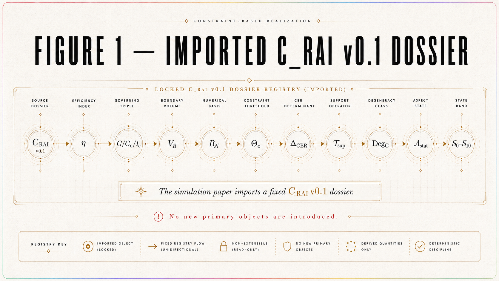
Figure 2 — Simulation Verdict Engine

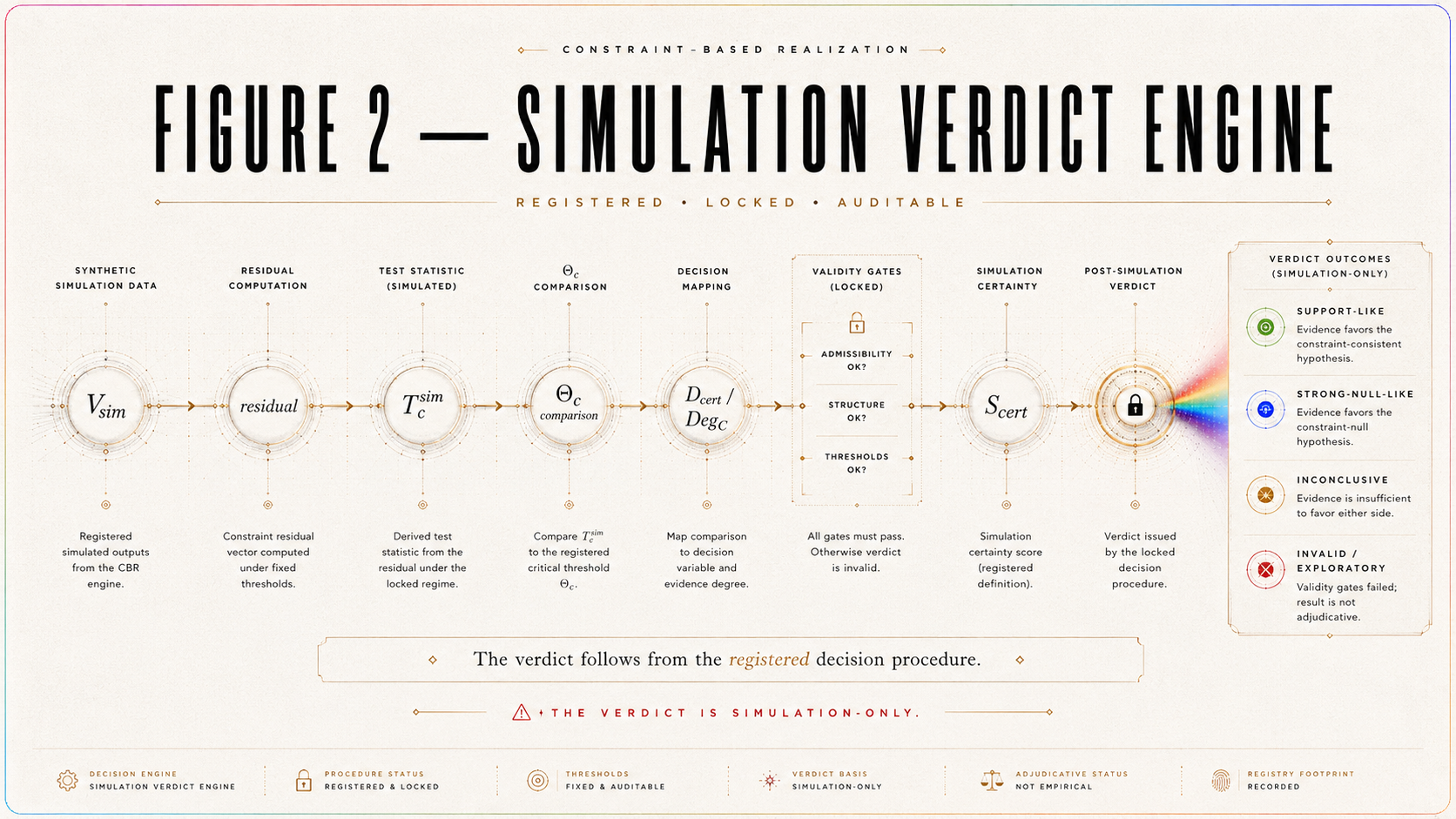
Figure 3 — Pre/Post Simulation Separation

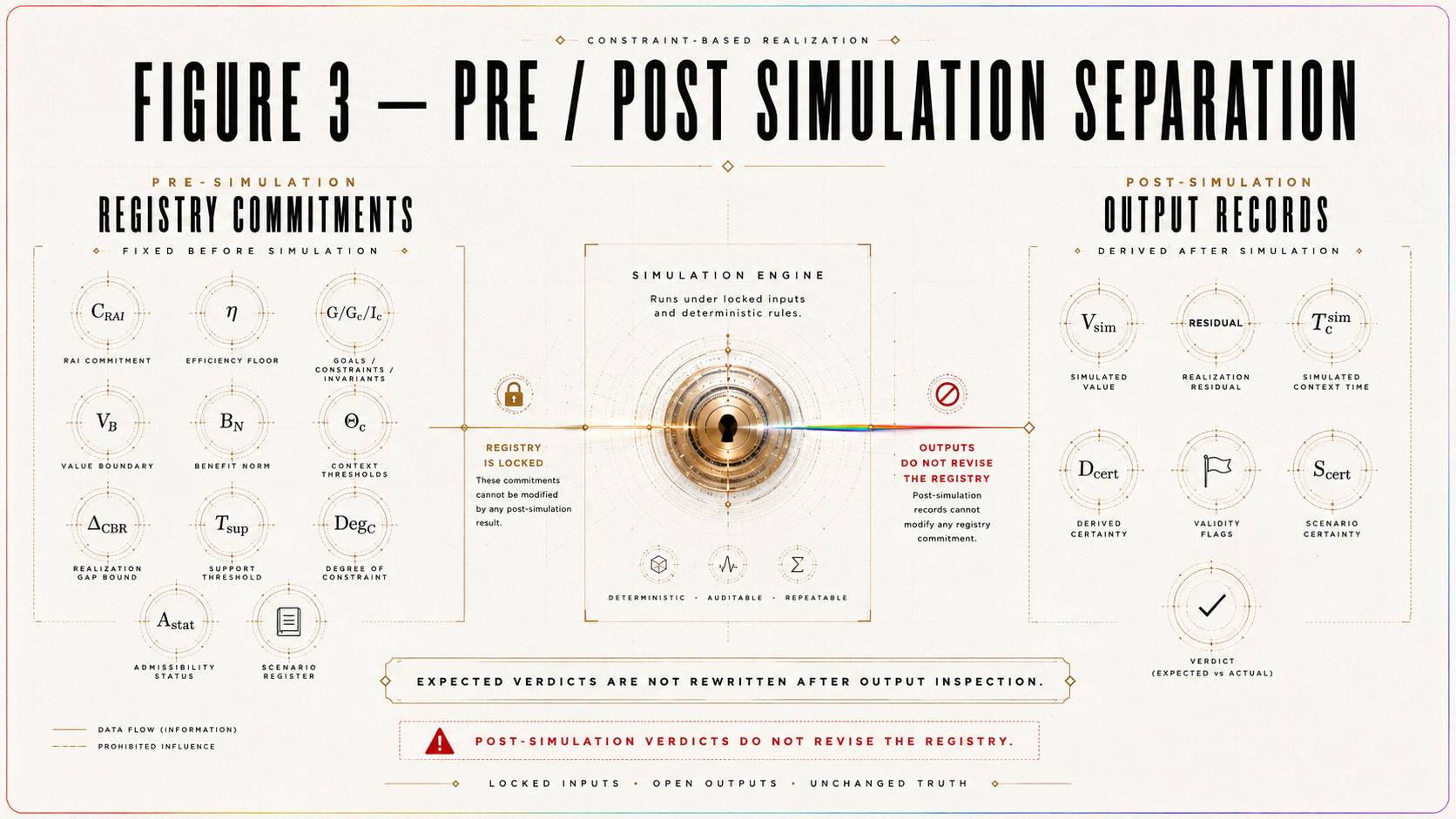
Figure 4 — Worked Demonstration Case

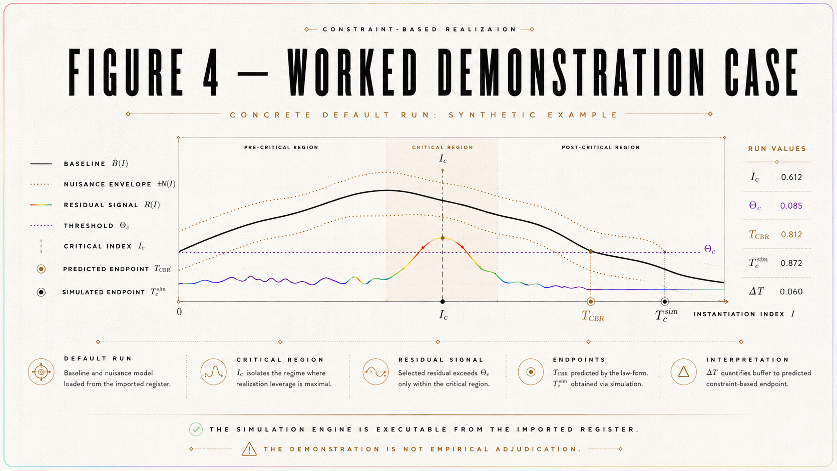
Figure 5 — Scenario Map S₀–S₁₀

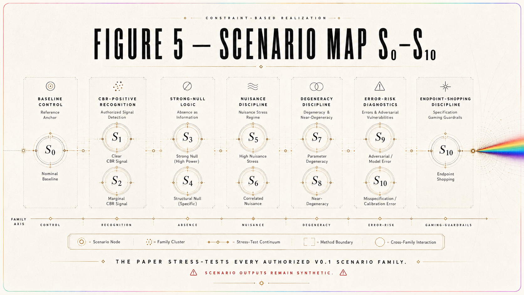
Figure 6 — Baseline / Residual / Nuisance Curves

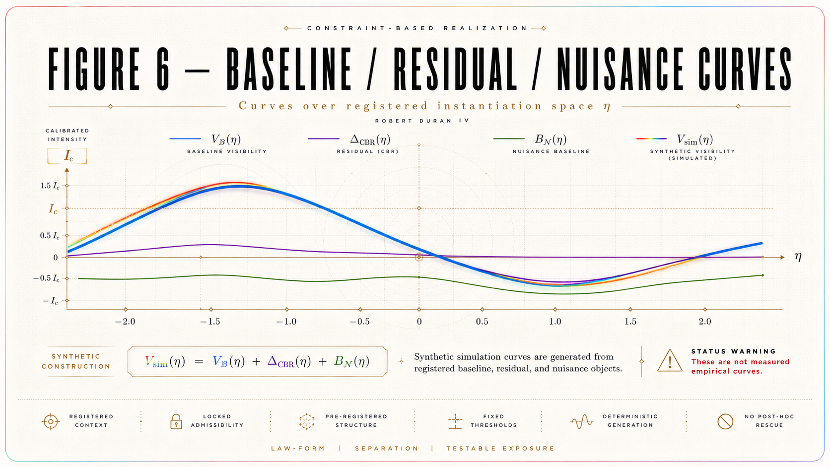
Figure 7 — Cross-Scenario Verdict Map

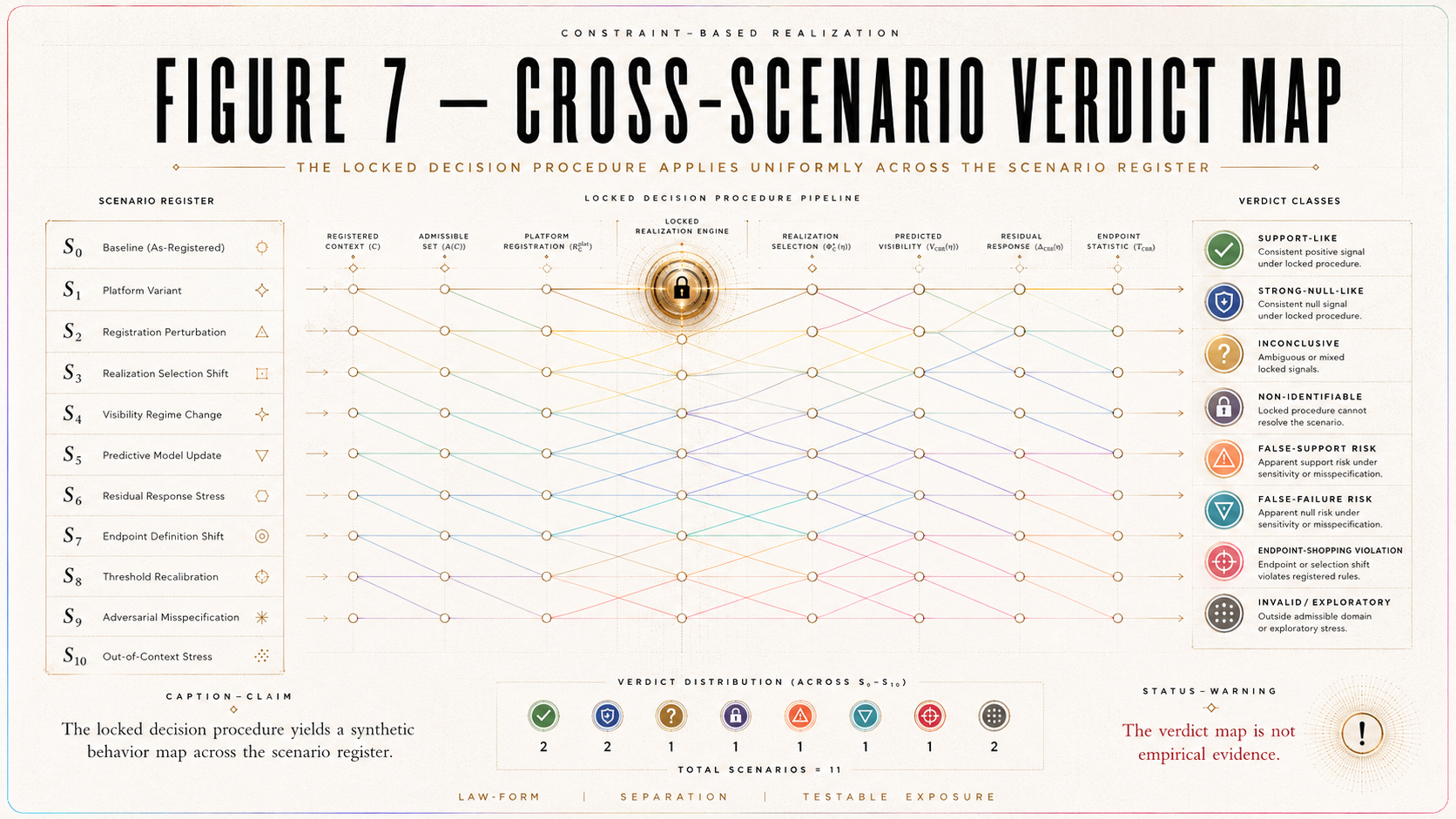
Figure 8 — Sensitivity Landscape

Figure 9 — False-Support and False-Failure Risk

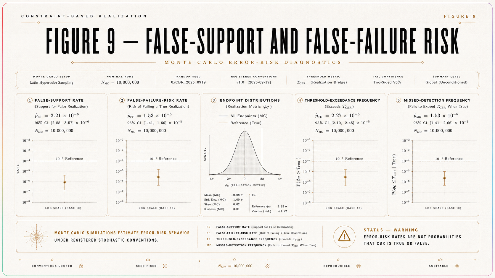
Figure 10 — Empirical Design Translation

---

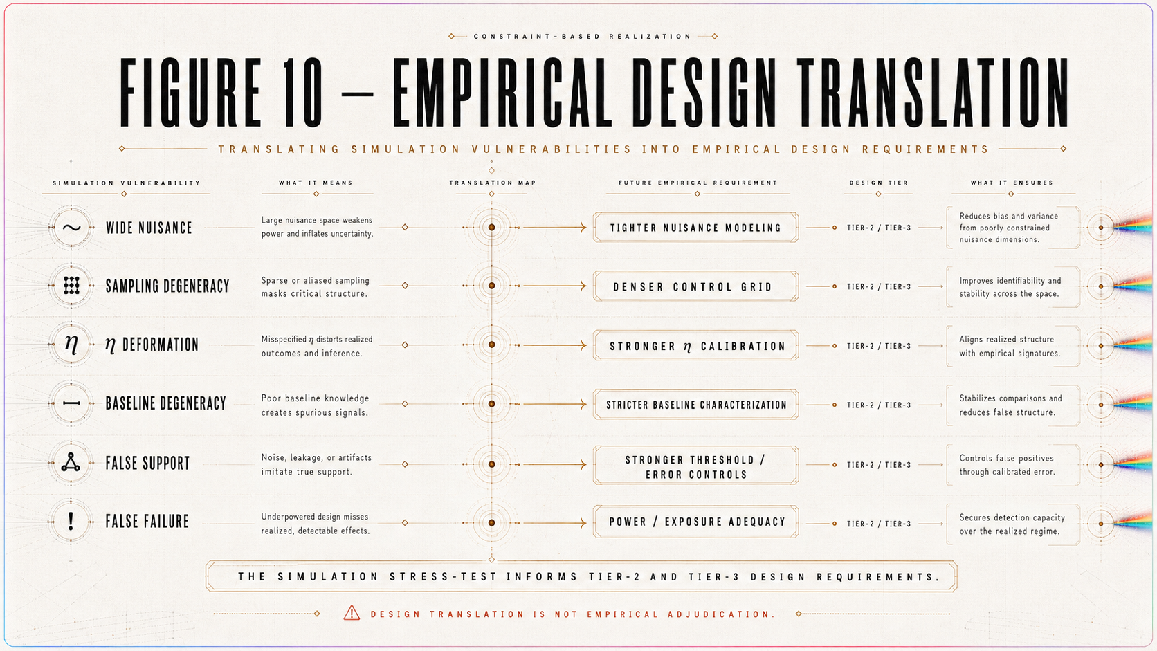
25. What This Paper Establishes

25.1 Establishment Statement

This paper establishes the simulation behavior of the locked C_RAI v0.1 decision procedure.

It establishes:

endpoint computability,
verdict-engine executability,
scenario-certificate use,
output-register traceability,
reproducibility discipline,
worked demonstration behavior,
deterministic rule behavior,
Monte Carlo error-risk behavior,
degeneracy-certificate use,
support-like simulation behavior,
strong-null-like simulation behavior,
inconclusive simulation behavior,
non-identifiable simulation behavior,
false-support risk behavior,
false-failure risk behavior,
endpoint-shopping discipline,
sensitivity profile,
and empirical-design lessons.

The paper establishes these objects synthetically. It does not establish empirical support or empirical failure.

25.2 What “Simulation Behavior” Means

Simulation behavior means the way the registered decision procedure classifies synthetic runs generated from the imported C_RAI v0.1 dossier.

It includes:

how endpoints are computed,
how thresholds are applied,
how degeneracy blocks identifiability,
how validity gates block overclaiming,
how baseline-only cases are classified,
how detectable synthetic residuals are recognized,
how below-threshold residuals become inconclusive,
how strong-null-like logic operates,
how nuisance produces inconclusiveness,
how baseline, η, and sampling degeneracies defeat identification,
how false-support risk appears,
how false-failure risk appears,
and how endpoint-shopping is prevented.

This is a decision-procedure result, not a physical discovery.

25.3 Proposition — Simulation Behavior Map

Proposition 25.1 — Simulation Behavior Map.
Given the imported C_RAI v0.1 dossier and authorized scenarios S₀–S₁₀, the paper establishes a complete synthetic behavior map for the registered endpoint, threshold, degeneracy, statistical, validity-gate, scenario-certificate, output-register, and verdict rules.

Proof Sketch

The imported dossier supplies all primary objects. The scenario register supplies all authorized test regimes. The simulation method computes endpoints, thresholds, degeneracy certificates, scenario certificates, output records, and verdicts. The cross-scenario verdict matrix consolidates those outputs, while sensitivity analysis identifies stability and fragility across registered variations. Therefore, the paper establishes how the locked decision machinery behaves under its declared synthetic regime.

25.4 What the Paper Establishes for CBR

The paper establishes that CBR’s C_RAI v0.1 platform dossier can be:

imported,
simulated,
stress-tested,
audited,
diagnosed,
sensitivity-tested,
error-risk-tested,
and translated into empirical design requirements.

This is a meaningful programmatic advance because it shows that the CBR platform instantiation is not merely a registry. It can be executed as a synthetic decision procedure.

25.5 What the Paper Establishes for Future Work

For future Tier-2 author-data reconstruction, the paper identifies the data and metadata needed to move beyond simulation.

For future Tier-3 locked experimentation, the paper identifies the calibration, nuisance, sampling, degeneracy, endpoint, and statistical requirements needed for meaningful empirical adjudication.

The paper therefore functions as a bridge from platform-specific numerical instantiation to empirical design.

The strongest successor work is not another simulation-only verdict, but either:

a Tier-2 author-data reconstruction with raw counts, calibrated uncertainties, covariance information, detector metadata, and dataset-specific nuisance modeling,

or:

a Tier-3 locked empirical dossier with pre-registered η, I_c, V_ℬ, B_𝓝, Θ_c, Δ_CBR, T_CBR, Deg_C, A_stat, validity gates, and verdict rules.

25.6 Establishment Boundary

The paper does not establish that CBR is true.

It does not establish empirical support.

It does not establish empirical failure.

It does not establish direct access to realization.

It does not establish that a CBR residual exists in nature.

It does not establish that ordinary quantum theory is false.

The final establishment is therefore precise:

The paper establishes a complete synthetic stress-test and behavior map of the locked C_RAI v0.1 decision procedure.

It does not establish empirical adjudication.

25.7 Boundary Principle

Principle 25.1 — Synthetic Establishment Boundary.
A simulation paper may establish the behavior, vulnerabilities, and empirical-design implications of a registered decision procedure, but it does not establish the truth, empirical support, or empirical failure of the physical law candidate.

25.8 Transition

The final section of the paper should state what the simulation study does not establish and then close with the paper’s final status:

simulation-executed, decision-procedure stress-tested, empirically non-adjudicative.

26. What This Paper Does Not Establish

26.1 Non-Establishment Statement

This paper establishes the synthetic behavior of the locked C_RAI v0.1 decision procedure. It does not establish the physical truth of Constraint-Based Realization.

It does not establish that CBR is true.

It does not establish that CBR is empirically confirmed.

It does not establish that CBR has failed.

It does not establish that realization has been directly observed.

It does not establish that any public dataset supports CBR.

It does not establish that ordinary quantum theory is false.

It does not establish empirical support.

It does not establish empirical failure.

These exclusions are not weaknesses in the paper’s design. They are the conditions that prevent the simulation study from overclaiming its evidential status. The paper is a simulation stress-test of a registered decision procedure, not an empirical adjudication of nature.

26.2 Non-Establishment of Empirical Adjudication

The paper uses synthetic simulations generated from the imported C_RAI v0.1 dossier. Therefore, every verdict category remains simulation-bound.

A positive synthetic result is:

simulation-only support-like

not empirical support.

A strong-null synthetic result is:

simulation-only strong-null-like

not empirical failure.

A false-support result is:

decision-procedure false-support risk

not evidence that CBR is supported.

A false-failure result is:

decision-procedure false-failure risk

not evidence that CBR is protected from failure.

A non-identifiable result is:

simulation-only non-identifiability

not a proof that CBR is untestable.

An inconclusive result is:

simulation-only inconclusiveness

not a failure of the broader realization-law thesis.

The paper therefore does not move from simulation to empirical verdict. It moves from locked platform dossier to executable decision-procedure behavior map.

26.3 Why Simulation Cannot Establish Realization

The CBR law-form concerns outcome realization. The present paper does not measure realization directly, nor does it claim that realization is directly observable in the simulation environment.

The simulation constructs synthetic baselines, nuisance terms, residuals, endpoints, degeneracy certificates, validity gates, and verdict classifications. These objects test the registered decision procedure. They do not show that nature realizes outcomes through the simulated residual family.

A simulation may show that a rule is coherent, fragile, conservative, over-sensitive, under-sensitive, or design-relevant. It cannot, by itself, show that the world instantiates the law-candidate being simulated.

Thus, even a clean support-like simulation outcome means only:

The decision procedure recognizes a detectable, non-degenerate synthetic residual under registered conditions.

It does not mean:

Nature contains the residual.

Likewise, a clean strong-null-like simulation outcome means only:

The decision procedure would classify a valid non-observation of a detectable, non-degenerate prediction as failure-like.

It does not mean:

CBR has failed empirically.

26.4 Non-Establishment of Public-Data Support

The preceding platform-specific numerical instantiation included a public-data pilot reconstruction. The present simulation paper may inherit that context programmatically, but it does not convert public-data pilot contact into empirical support.

Pilot reconstruction and simulation stress-testing have different statuses.

A pilot reconstruction demonstrates that endpoint computation can be applied to public data under declared assumptions.

A simulation stress-test demonstrates that the registered decision procedure behaves in certain ways under synthetic conditions.

Neither is a registered empirical test unless the relevant empirical objects are calibrated, validated, and pre-registered.

Therefore, this paper does not claim that any public dataset supports CBR.

26.5 Non-Establishment of Failure

The paper also does not fail CBR.

A simulation-only strong-null-like result may show that the verdict engine can issue a failure-like classification under synthetic conditions. But empirical failure would require more than simulation.

It would require, at minimum:

calibrated η,
fixed I_c,
validated V_ℬ(η),
validated B_𝓝(η),
pre-registered Δ_CBR(η),
computed T_CBR,
implemented Deg_C,
implemented A_stat,
adequate sampling,
valid exposure,
and a real empirical endpoint satisfying the registered failure condition.

Without these conditions, strong-null-like simulation remains procedural, not empirical.

26.6 Non-Establishment of Standard Quantum Failure

The paper does not establish that ordinary quantum theory is false.

The ordinary baseline V_ℬ and nuisance envelope B_𝓝 are part of the simulation architecture. They represent synthetic comparators and ordinary allowances inside the C_RAI v0.1 stress-test. They are not a full experimental challenge to standard quantum theory.

Even if a synthetic residual exceeds a threshold in simulation, this does not imply that standard quantum mechanics has failed. It implies only that the decision rule classifies that synthetic construction in a particular way.

Empirical challenge to ordinary quantum predictions would require a separate locked empirical dossier with validated ordinary modeling, calibrated apparatus information, uncertainty propagation, nuisance modeling, and pre-registered verdict rules.

26.7 Non-Establishment of Universality

This paper does not establish a universal CBR law, a universal Born-rule derivation, or a universal empirical signature across all possible measurement contexts.

The scope is limited to:

C_RAI v0.1,
the imported record-accessibility interferometric context,
the registered synthetic residual family,
the registered baseline and nuisance structures,
the registered endpoint 𝒯_sup,
and the authorized scenario set S₀–S₁₀.

Any claim beyond that scope would require a successor paper, successor dossier, or additional theorem.

26.8 Simulation Status Discipline

Principle 26.1 — Simulation Status Discipline.
A simulation may test the behavior of a registered decision procedure, but it cannot establish that nature realizes the simulated residual.

This principle governs every result in the paper.

It applies to support-like outcomes.

It applies to strong-null-like outcomes.

It applies to false-support and false-failure diagnostics.

It applies to sensitivity runs.

It applies to design recommendations.

No simulation result is permitted to become empirical adjudication by implication, rhetoric, figure design, or summary language.

26.9 Final Non-Establishment Boundary

The final non-establishment boundary is therefore:

This paper establishes how the locked C_RAI v0.1 decision procedure behaves under synthetic stress-testing. It does not establish whether CBR is true, supported, failed, observed, or physically instantiated.

That boundary is not a retreat from the paper’s contribution. It is what makes the contribution exact.

26.10 Transition

The conclusion states the final status of the simulation paper.

27. Conclusion

27.1 Summary

This paper imports the locked C_RAI v0.1 dossier and stress-tests its decision procedure across the authorized scenario register S₀–S₁₀.

It tests:

detectability,
threshold behavior,
degeneracy behavior,
strong-null logic,
nuisance sensitivity,
baseline mimicry,
η-calibration sensitivity,
sampling adequacy,
false-support risk,
false-failure risk,
endpoint-shopping discipline,
cross-scenario verdict consistency,
sensitivity robustness,
and empirical-design translation.

The paper does not revise the imported dossier. It does not introduce new primary test objects. It does not change the endpoint after seeing results. It does not convert secondary diagnostics into primary verdict criteria. It does not convert simulation-only classifications into empirical verdicts.

Its object is the registered C_RAI v0.1 decision machinery.

27.2 Main Achievement

The main achievement is not empirical confirmation.

The main achievement is a complete synthetic behavior map of the locked C_RAI v0.1 verdict machinery.

The paper shows how the decision procedure behaves when:

no CBR residual is present,
a detectable synthetic residual is present,
a residual is below threshold,
a detectable prediction fails to appear under valid exposure,
wide nuisance blocks separation,
ordinary baseline variation mimics the residual,
η uncertainty defeats identification,
sampling fails to resolve the residual,
ordinary noise creates false-support risk,
inadequate exposure creates false-failure risk,
and secondary endpoints attempt to rescue a primary-endpoint failure.

The central result is therefore procedural rather than empirical:

C_RAI v0.1 is not merely a locked dossier. It is an executable decision procedure whose behavior can be simulated, audited, stress-tested, and translated into future empirical design requirements.

27.3 Programmatic Significance

This paper advances the CBR program by moving from platform registration to simulation execution.

Earlier CBR works supplied the conceptual burden, canonical law-form, accessibility endpoint logic, failure discipline, jurisdiction rules, and platform-specific dossier. The present paper tests whether the platform-specific dossier behaves coherently under the scenario classes it authorizes.

The programmatic significance is therefore structural.

CBR’s platform dossier can now be:

simulated,
stress-tested,
audited,
diagnosed,
limited,
sensitivity-tested,
error-risk-tested,
and used to guide empirical design.

This is a meaningful step because it shows that the CBR framework can be developed as a disciplined research program rather than as a merely interpretive statement.

27.4 Empirical Design Significance

The paper’s empirical value is not that it provides empirical support. It does not.

Its empirical value is that it identifies what a future empirical dossier must control.

The simulation results specify the kinds of requirements needed for Tier-2 and Tier-3 work:

raw phase-scan data,
calibrated η,
fixed I_c,
validated baseline modeling,
validated nuisance envelopes,
adequate sampling density,
uncertainty propagation,
degeneracy checks,
threshold margins,
endpoint hierarchy,
statistical rule implementation,
and pre-registered verdict criteria.

Thus, the paper’s empirical contribution is preparatory and design-facing.

It does not answer:

Is CBR confirmed?

It answers:

What must be true of a future empirical test before CBR could be meaningfully supported or failed?

27.5 Relationship to the Prior Paper

The prior paper constructed the locked C_RAI v0.1 numerical dossier.

The present paper executes that dossier in simulation.

The relationship may be summarized as follows:

Platform-specific numerical instantiation fixes the machine.

Simulation scenarios test the machine.

The first paper defines the registered objects.

The second paper evaluates the behavior of the registered decision procedure under controlled synthetic conditions.

Together, they move CBR from abstract law-form and empirical aspiration toward executable pre-empirical methodology.

27.6 Relationship to Future Work

The strongest successor work is not another simulation-only verdict.

The strongest successor work is one of two things.

First:

a Tier-2 author-data reconstruction

using raw counts, uncertainty estimates, detector metadata, calibration information, covariance structure, phase-scan data, and dataset-specific nuisance modeling.

Second:

a Tier-3 locked empirical dossier

with pre-registered η, I_c, V_ℬ, B_𝓝, Θ_c, Δ_CBR, T_CBR, Deg_C, A_stat, validity gates, endpoint hierarchy, and verdict rules.

This simulation paper prepares those successor steps by identifying the design vulnerabilities that must be controlled.

27.7 Final Status

Before simulations are executed, the paper’s design status is:

simulation-ready decision-procedure stress test.

After simulations are completed, output records are generated, scenario certificates are assigned, and verdict behavior is reported, the paper’s final status becomes:

simulation-executed, decision-procedure stress-tested, empirically non-adjudicative.

The final status statement for the completed paper is:

This paper establishes a complete synthetic stress-test of the locked C_RAI v0.1 decision procedure across the authorized scenario register S₀–S₁₀. It demonstrates simulation execution, verdict traceability, error-risk diagnostics, sensitivity profiling, endpoint discipline, and empirical-design translation. It does not establish empirical support, empirical failure, or the truth of CBR.

27.8 Closing Statement

Constraint-Based Realization treats outcome realization as a distinct explanatory target from probability assignment, decoherent record formation, and ordinary measurement registration. The present paper does not settle that target. It does not claim that the realization law has been observed.

Its contribution is narrower and stricter.

It shows that a registered CBR platform dossier can be taken seriously as an executable object: fixed before simulation, run through authorized scenarios, checked against validity and degeneracy rules, protected against false support and false failure, and translated into future empirical requirements.

That is the paper’s final contribution:

not confirmation, not failure, but disciplined execution.

Appendix A — Imported C_RAI v0.1 Register

A.1 Purpose

This appendix collects the imported C_RAI v0.1 objects used throughout the simulation paper.

The purpose is to make the simulation boundary explicit. The main text repeatedly relies on the rule that this paper imports rather than revises the platform-specific dossier. This appendix lists the imported objects so that the reader can verify what belongs to v0.1, what may be varied inside v0.1, and what would require a successor version.

A simulation remains inside C_RAI v0.1 only if it uses the imported objects or authorized scenario variations. Any change to a primary object creates an exploratory variation, an outside-v0.1 stress test, or a successor dossier.

A.2 Platform Context

The imported context is:

C_RAI = record-accessibility interferometric context.

This context is the platform class for the simulation stress-test.

It is not a claim that the simulated residual exists in an empirical interferometer. It is the declared platform context for the synthetic decision procedure.

A.3 Accessibility Register

The imported accessibility variable is:

η ∈ [0,1].

The imported accessibility grid is:

G = {η_j = j/(N_η − 1) : j = 0, …, N_η − 1}.

The default grid size is:

N_η = 101.

The imported critical regime is:

I_c = [0.4, 0.6].

The grid-restricted critical regime is:

G_c = G ∩ I_c.

The accessibility variable is simulation-registered, not empirically calibrated in this paper.

A.4 Baseline Register

The imported ordinary baseline class is:

𝔅 = {V_ℬ(η; θ_ℬ) : θ_ℬ ∈ Θ_ℬ}.

The imported baseline form is:

V_ℬ(η; θ_ℬ) = V₀(1 − qη)exp(−κη)(1 − ρη) + λ₀ + λ₁η.

The central baseline parameter vector is:

θ_ℬ⁰ = (V₀, q, κ, ρ, λ₀, λ₁) = (0.90, 0.10, 0.20, 0.03, 0, 0).

The registered parameter ranges are:

V₀ ∈ [0.75, 1.00],

q ∈ [0, 0.30],

κ ∈ [0, 0.50],

ρ ∈ [0, 0.10],

λ₀ ∈ [−0.01, 0.01],

λ₁ ∈ [−0.02, 0.02].

All baseline simulations must preserve:

0 ≤ V_ℬ(η; θ_ℬ) ≤ 1

on the relevant grid, up to registered numerical tolerance.

A.5 Nuisance Register

The imported nuisance regimes are:

B_𝓝^narrow = 0.0075,

B_𝓝^moderate = 0.0175,

B_𝓝^wide = 0.0375.

The central nuisance regime is:

B_𝓝^moderate.

The nuisance realization in simulation is denoted:

δ_𝓝(η).

The nuisance envelope B_𝓝(η) defines ordinary allowance. The realized nuisance δ_𝓝(η) defines a simulated perturbation inside a run.

A.6 Threshold Register

The imported critical nuisance bound is:

B_c = sup_{η ∈ I_c} B_𝓝(η).

On the grid:

B_c^G = max_{η_j ∈ G_c} B_𝓝(η_j).

The imported detectability threshold is:

ε_detect = z_detect σ_T.

The imported decision threshold is:

Θ_c = B_c + ε_detect.

Central simulations use:

z_detect = 2.

Conservative stress tests may use:

z_detect = 3.

For symbolic demonstrations, Θ_c may remain symbolic. For numerical runs, σ_T, ε_detect, and Θ_c must be instantiated and reported in the output register.

A.7 Residual Register

The imported synthetic CBR residual family is:

Δ_CBR(η) = A_CBR s exp[−(η − η_c)²/(2w_r²)].

The central residual location is:

η_c = 0.5.

The registered width family is:

w_r ∈ {0.025, 0.05, 0.10}.

The registered sign family is:

s ∈ {+1, −1}.

The registered amplitude family is:

A_CBR ∈ {0, 0.5Θ_c, Θ_c, 1.5Θ_c, 2Θ_c, 3Θ_c}.

This residual family is synthetic. It is used to test decision-procedure behavior, not to claim empirical discovery.

A.8 Endpoint Register

The imported primary endpoint is:

𝒯_sup[x(η), η ∈ I_c] = sup_{η ∈ I_c}|x(η)|.

On the grid:

𝒯_sup^G[x] = max_{η_j ∈ G_c}|x(η_j)|.

The predicted endpoint is:

T_CBR = 𝒯_sup[Δ_CBR(η), η ∈ I_c].

The simulated endpoint is:

T_c^sim = 𝒯_sup[V_sim(η) − V_ℬ(η), η ∈ I_c].

The primary endpoint hierarchy is:

𝒯_sup first, registered diagnostics second, exploratory endpoints only in successor versions.

A.9 Degeneracy Register

The imported degeneracy operator is:

Deg_C = Deg_𝔅 ∪ Deg_𝓝 ∪ Deg_η ∪ Deg_est ∪ Deg_post ∪ Deg_phase ∪ Deg_samp ∪ Deg_stat ∪ Deg_end.

The imported degeneracy certificate is:

Dcert(Δ_CBR).

Allowed statuses are:

non-degenerate,
degenerate,
not evaluable,
requires future testing.

Support-like and strong-null-like classification require:

Dcert(Δ_CBR) = non-degenerate.

A.10 Statistical and Verdict Register

The imported statistical rule is:

A_stat.

In v0.1, the primary convention is the envelope-threshold rule using Θ_c.

The registered verdict categories are:

simulation-only support-like,
simulation-only strong-null-like,
simulation-only inconclusive,
simulation-only non-identifiable,
false-support risk,
false-failure risk,
endpoint-shopping violation,
invalid scenario,
and exploratory outside-v0.1.

A.11 Scenario Register

The authorized scenario classes are:

S₀ — baseline-only control,
S₁ — detectable CBR-positive case,
S₂ — undetectable CBR-positive case,
S₃ — strong-null scenario,
S₄ — wide-nuisance inconclusiveness,
S₅ — baseline degeneracy,
S₆ — η-miscalibration,
S₇ — sampling degeneracy,
S₈ — false-support stress test,
S₉ — false-failure stress test,
S₁₀ — endpoint-shopping stress test.

A.12 Fixed and Varied Objects

The imported register contains both fixed objects and registered variation objects.

The fixed objects include:

C_RAI,
the primary endpoint 𝒯_sup,
the scenario register S₀–S₁₀,
the registered verdict categories,
the no-new-primary-objects rule,
the pre/post simulation separation rule,
the output-register requirement,
and the version-boundary rule.

The registered variation objects include:

A_CBR,
w_r,
s,
B_𝓝 regime,
τ_deg,
grid density,
registered η deformations,
and z_detect.

A variation of a registered variation object may remain inside C_RAI v0.1 if it stays within the declared range or authorized stress condition.

A change to a fixed object creates an exploratory analysis or successor version unless explicitly authorized by the imported register.

A.13 Register Boundary

Principle A.1 — Imported Register Boundary.
The objects listed in Appendix A define the imported C_RAI v0.1 simulation register. A run that changes a primary object is not a registered v0.1 run unless the change is explicitly declared as an authorized sensitivity condition.

Appendix B — Simulation Algorithm

B.1 Purpose

This appendix states the executable simulation algorithm.

The purpose is to make the path from imported dossier to post-simulation verdict explicit. A reader should be able to reconstruct every reported verdict by following the algorithm, checking the output register, and verifying the scenario certificate.

The algorithm does not revise the dossier. It implements it.

B.2 Algorithm Overview

For each simulation run, the algorithm proceeds as follows:

import the C_RAI v0.1 dossier,
declare scenario S_i,
load fixed objects,
load varied objects,
instantiate the parameter state,
generate baseline V_ℬ(η),
generate nuisance δ_𝓝(η),
generate residual Δ_CBR(η),
compute simulated visibility V_sim(η),
compute T_CBR,
compute T_c^sim,
compute B_c, ε_detect, and Θ_c,
compute or assign Dcert,
generate Scert,
apply validity gates,
classify the post-simulation verdict,
record the output,
and update scenario-level summaries.

B.3 Step 1 — Import Dossier

The algorithm begins by importing the objects listed in Appendix A.

No primary object may be changed during import.

If the run requires a new primary object, the run must be labeled:

exploratory outside v0.1,
stress test outside v0.1,
or successor dossier required.

B.4 Step 2 — Declare Scenario

Choose the scenario:

S_i ∈ {S₀, S₁, …, S₁₀}.

Record:

scenario ID,
scenario purpose,
expected verdict family,
fixed objects,
varied objects,
and version status.

The expected verdict must be declared before simulation.

B.5 Step 3 — Instantiate Parameters

Instantiate all required parameters:

baseline parameter vector θ_ℬ,
nuisance regime B_𝓝,
nuisance realization rule,
residual amplitude A_CBR,
residual width w_r,
residual sign s,
grid density N_η,
critical regime I_c,
degeneracy tolerance τ_deg,
statistical setting z_detect,
and any scenario-specific deformation or stress condition.

For stochastic runs, also instantiate:

N_MC,
seed list or seed-generation rule,
and nuisance sampling convention.

B.6 Step 4 — Generate Baseline

Compute:

V_ℬ(η; θ_ℬ)

on the simulation grid.

Check physical admissibility:

0 ≤ V_ℬ(η; θ_ℬ) ≤ 1.

If the baseline violates admissibility, the run fails the baseline admissibility gate.

B.7 Step 5 — Generate Nuisance

Generate or assign:

δ_𝓝(η).

For deterministic runs, this may be zero or a controlled construction.

For stochastic runs, this is sampled under the registered nuisance convention.

The nuisance realization must be recorded.

The nuisance non-duplication gate must be checked to ensure nuisance is not double-counted against the baseline model.

B.8 Step 6 — Generate Residual

Generate:

Δ_CBR(η) = A_CBR s exp[−(η − η_c)²/(2w_r²)].

For scenarios where no CBR residual is present, set:

Δ_CBR(η) = 0.

For strong-null scenarios, distinguish the prediction-side residual from the simulation-side visibility construction.

B.9 Step 7 — Compute Simulated Visibility

Compute:

V_sim(η) = V_ℬ(η) + Δ_CBR(η) + δ_𝓝(η).

If the scenario intentionally omits the predicted residual from simulated visibility, as in a strong-null construction, record that distinction explicitly.

Check physical admissibility:

0 ≤ V_sim(η) ≤ 1.

For default v0.1 runs, invalidation is preferred over post hoc clipping unless clipping is explicitly pre-registered.

B.10 Step 8 — Compute Endpoints

Compute:

T_CBR = 𝒯_sup[Δ_CBR(η), η ∈ I_c].

Compute:

T_c^sim = 𝒯_sup[V_sim(η) − V_ℬ(η), η ∈ I_c].

All endpoint values must be recorded in the output register.

B.11 Step 9 — Compute Threshold

Compute:

B_c = sup_{η ∈ I_c} B_𝓝(η).

Compute:

ε_detect = z_detect σ_T.

Compute:

Θ_c = B_c + ε_detect.

If σ_T remains symbolic, the run must report threshold relationships symbolically. If the run is numerical, σ_T, ε_detect, and Θ_c must be numerically instantiated.

B.12 Step 10 — Evaluate Degeneracy

Compute or assign:

Dcert(Δ_CBR).

Check whether the residual belongs to:

Deg_𝔅,
Deg_𝓝,
Deg_η,
Deg_est,
Deg_post,
Deg_phase,
Deg_samp,
Deg_stat,
or Deg_end.

If degeneracy is triggered, support-like and strong-null-like verdicts are unavailable.

B.13 Step 11 — Apply Validity Gates

Evaluate:

endpoint congruence,
sampling adequacy,
baseline admissibility,
nuisance non-duplication,
threshold computability,
degeneracy evaluability,
registered statistical rule,
provenance consistency,
and version consistency.

Each gate must be recorded as:

pass,
fail,
not applicable,
or not evaluable.

B.14 Step 12 — Generate Scenario Certificate

Generate:

Scert(S_i).

The scenario certificate records:

fixed objects,
varied objects,
variation ranges,
provenance,
expected verdict,
post-simulation verdict,
validity status,
degeneracy status,
and version status.

A run without Scert(S_i) is not a registered v0.1 run.

B.15 Step 13 — Classify Verdict

Classify the post-simulation verdict as one of:

simulation-only support-like,
simulation-only strong-null-like,
simulation-only inconclusive,
simulation-only non-identifiable,
false-support risk,
false-failure risk,
endpoint-shopping violation,
invalid scenario,
or exploratory outside-v0.1.

The verdict must follow the registered rule. It cannot be chosen after narrative interpretation.

B.16 Step 14 — Record Output

Write the output record containing:

scenario ID,
run ID,
seed or deterministic label,
parameter state,
endpoint values,
threshold values,
certificates,
validity gates,
expected verdict,
post-simulation verdict,
and version status.

No numerical result may be reported in the paper unless it is traceable to such a record.

B.17 Algorithm Failure Rule

If any required object is missing, non-computable, inconsistent, outside the imported register, or unavailable under the declared scenario, the algorithm must stop and classify the run as one of the following:

invalid,
not evaluable,
exploratory outside v0.1,
or successor version required.

The algorithm may not silently impute a missing object, alter the endpoint, adjust the threshold, widen or narrow the nuisance envelope, substitute a new baseline class, or repair the scenario after observing output.

B.18 Algorithmic Principle

Principle B.1 — Algorithmic Traceability.
Every reported simulation verdict must be reproducible from the imported dossier, scenario declaration, parameter state, endpoint computation, threshold computation, certificates, validity gates, and output record.

Appendix C — Worked Demonstration Output

C.1 Purpose

This appendix records the complete worked demonstration output from Section 5.

The purpose is to provide one concrete example of the simulation engine in operation. The demonstration is not empirical. It is a rule-behavior example showing how imported objects, simulated visibility, endpoint computation, threshold comparison, certificates, validity gates, and verdict classification fit together.

C.2 Demonstration Run D₀

The main demonstration run is:

D₀ = central deterministic recognition demonstration.

The construction label is:

central deterministic recognition demonstration.

The scenario relation is:

linked to S₁, because it demonstrates recognition of a detectable synthetic residual.

This naming is deliberate. The run demonstrates support-like recognition behavior inside a synthetic decision procedure. It does not demonstrate empirical support.

C.3 Imported Central Values

The demonstration uses:

N_η = 101,

I_c = [0.4, 0.6],

V₀ = 0.90,

q = 0.10,

κ = 0.20,

ρ = 0.03,

λ₀ = 0,

λ₁ = 0,

B_𝓝 = B_𝓝^moderate = 0.0175,

η_c = 0.5,

w_r = 0.05,

s = +1.

The realized nuisance is:

δ_𝓝(η) = 0.

The residual amplitude is:

A_CBR = 1.5Θ_c.

C.4 Baseline

The central baseline is:

V_ℬ⁰(η) = 0.90(1 − 0.10η)exp(−0.20η)(1 − 0.03η).

This baseline is synthetic and simulation-registered.

It is not fitted to empirical data.

C.5 Residual

The demonstration residual is:

Δ_CBR^D₀(η) = 1.5Θ_c exp[−(η − 0.5)²/(2 · 0.05²)].

Since:

η_c = 0.5 ∈ I_c,

the predicted endpoint is:

T_CBR^D₀ = 1.5Θ_c.

Therefore:

T_CBR^D₀ > Θ_c.

C.6 Simulated Visibility

The simulated visibility is:

V_sim^D₀(η) = V_ℬ⁰(η) + Δ_CBR^D₀(η).

The simulated residual relative to baseline is:

V_sim^D₀(η) − V_ℬ⁰(η) = Δ_CBR^D₀(η).

Therefore:

T_c^sim,D₀ = 1.5Θ_c.

Thus:

T_c^sim,D₀ > Θ_c.

C.7 Certificates

The degeneracy certificate is:

Dcert(Δ_CBR^D₀) = non-degenerate

provided no baseline, nuisance, η, sampling, statistical, endpoint, or validity degeneracy is activated.

The scenario certificate is:

Scert(D₀) = valid central deterministic recognition demonstration

provided all validity gates pass.

C.8 Validity Gates

The validity-gate status for D₀ is:

endpoint congruence: pass,
sampling adequacy: pass under default grid and w_r = 0.05,
baseline admissibility: pass if V_sim^D₀ ∈ [0,1],
nuisance non-duplication: pass,
threshold computability: pass,
degeneracy evaluability: pass,
registered statistical rule: pass,
provenance consistency: pass,
version consistency: pass.

If physical admissibility fails for a numerical instantiation of Θ_c, the demonstration run must be marked invalid or re-expressed using a lower registered amplitude. It may not be rescued by post hoc clipping unless clipping was pre-registered.

C.9 Demonstration Verdict

The expected verdict is:

support-like recognition demonstration.

The post-simulation verdict is:

simulation-only support-like recognition demonstration

provided validity gates pass.

This verdict is not empirical support. It demonstrates that the decision engine recognizes a detectable, non-degenerate synthetic residual under central deterministic conditions.

C.10 Optional Baseline-Only Demonstration Variant D₀′

The optional baseline-only demonstration variant is:

D₀′ = central deterministic baseline-only demonstration.

Set:

A_CBR = 0

and:

δ_𝓝(η) = 0.

Then:

Δ_CBR^D₀′(η) = 0,

V_sim^D₀′(η) = V_ℬ⁰(η),

T_CBR^D₀′ = 0,

and:

T_c^sim,D₀′ = 0.

The expected verdict is:

simulation-only baseline / no-support.

The post-simulation verdict is:

simulation-only baseline / no-support

provided validity gates pass.

C.11 Demonstration Boundary

The worked demonstration does not establish CBR support.

It does not establish CBR failure.

It does not establish empirical adjudication.

It shows only that the registered simulation engine can be executed on a central deterministic case.

Principle C.1 — Demonstration Boundary.
A worked demonstration output illustrates the decision procedure. It does not supply empirical support, empirical failure, or evidence that nature realizes the simulated residual.

Appendix D — Simulation Output Register

D.1 Purpose

This appendix provides the required output schema for every simulation run.

The output register is the audit trail of the paper. It ensures that every reported verdict can be traced to the scenario, parameter state, endpoint computation, threshold computation, certificates, validity gates, expected verdict, post-simulation verdict, and version status.

A simulation result not recorded in this schema may be exploratory, but it may not support a reported finding.

D.2 Required Fields

Every output record must include:

scenario ID,
run ID,
seed or deterministic construction label,
baseline parameter vector,
nuisance regime,
nuisance realization label,
residual parameters,
grid parameters,
η-deformation parameters if applicable,
endpoint values,
threshold values,
degeneracy certificate,
scenario certificate,
validity-gate status,
expected verdict,
post-simulation verdict,
error-risk fields if applicable,
endpoint-shopping fields if applicable,
and version status.

D.3 Scenario and Run Identification

The output record must identify:

S_i ∈ {S₀, S₁, …, S₁₀}

and a unique run ID.

Examples:

S₀-D1 for deterministic baseline-only control.

S₁-D1 for deterministic support-like recognition.

S₈-MC-0001 for a Monte Carlo false-support run.

S₉-MC-0001 for a Monte Carlo false-failure run.

The run ID must be unique within the simulation package.

D.4 Parameter Fields

Each record must include:

θ_ℬ,
B_𝓝,
δ_𝓝 rule or realization label,
A_CBR,
w_r,
s,
η_c,
N_η,
G,
G_c,
I_c,
τ_deg,
z_detect,
σ_T if numerical,
and any scenario-specific deformation.

If a parameter is symbolic, the record must state that it is symbolic. If a parameter is numerical, its value must be recorded.

D.5 Endpoint Fields

Each record must include:

T_CBR,
T_c^sim,
B_c,
ε_detect,
and Θ_c.

It must also state whether:

T_CBR > Θ_c,
T_CBR = Θ_c,
T_CBR < Θ_c,
T_c^sim > Θ_c,
T_c^sim = Θ_c,
or T_c^sim < Θ_c.

The equality convention must be applied conservatively.

D.6 Certificate Fields

Each record must include:

Dcert(Δ_CBR)

with one of the registered statuses:

non-degenerate,
degenerate,
not evaluable,
or requires future testing.

Each record must also include:

Scert(S_i).

The scenario certificate must state:

fixed objects,
varied objects,
variation range,
provenance,
expected verdict,
post-simulation verdict,
validity status,
degeneracy status,
and version status.

D.7 Validity-Gate Fields

Each output record must report the status of:

endpoint congruence,
sampling adequacy,
baseline admissibility,
nuisance non-duplication,
threshold computability,
degeneracy evaluability,
registered statistical rule,
provenance consistency,
and version consistency.

Each gate must be labeled:

pass,
fail,
not applicable,
or not evaluable.

If a required gate fails, support-like and strong-null-like verdicts are unavailable.

D.8 Verdict Fields

Each record must contain:

expected verdict,
post-simulation verdict,
and verdict-family status.

The post-simulation verdict must be one of:

simulation-only support-like,
simulation-only strong-null-like,
simulation-only inconclusive,
simulation-only non-identifiable,
false-support risk,
false-failure risk,
endpoint-shopping violation,
invalid scenario,
or exploratory outside-v0.1.

No unregistered verdict category may be introduced inside the output record.

D.9 Error-Risk Fields

For false-support scenarios, record:

threshold-exceedance status,
false-support flag,
false-support rate if part of Monte Carlo summary,
nuisance regime,
maximum false endpoint if relevant,
and uncertainty interval or standard error if a rate is reported.

For false-failure scenarios, record:

missed-detection status,
false-failure-risk flag,
underpowering or exposure-adequacy diagnosis,
sampling-failure diagnosis,
nuisance-swallowing diagnosis,
η-miscalibration diagnosis if applicable,
and uncertainty interval or standard error if a rate is reported.

D.10 Endpoint-Shopping Fields

For endpoint-shopping scenarios, record:

primary endpoint value,
secondary endpoint value if used,
whether the secondary endpoint was registered,
whether the secondary endpoint is diagnostic or decisive,
whether endpoint-shopping was attempted,
and whether the run remains inside v0.1.

If a secondary endpoint is used decisively without prior registration, the run must be labeled:

endpoint-shopping violation

or:

exploratory outside-v0.1.

D.11 Version Fields

Each output record must state one of the following:

inside C_RAI v0.1,
registered v0.1 stress scenario,
exploratory outside v0.1,
successor version required,
or invalid.

A run cannot silently change status after output inspection.

D.12 Machine-Readable Format Recommendation

The preferred output-register format is machine-readable.

Suitable formats include:

CSV,
JSON,
structured spreadsheet,
or another version-controlled structured format.

The recommended structure is one row or record per run, linked to scenario-level summaries, parameter manifests, seed lists, and figure-generation inputs.

A machine-readable output register is not required for the conceptual validity of the paper, but it is strongly preferred for reproducibility, auditability, and future extension.

D.13 Output Register Principle

Principle D.1 — Output Register Completeness.
A simulation verdict is reportable only if the output record contains the scenario identity, parameter state, endpoint values, threshold values, certificates, validity-gate outcomes, expected verdict, post-simulation verdict, and version status required to reproduce and audit the classification.

D.14 Output Package Recommendation

A complete output package should include:

run-level output records,
scenario-level summaries,
Monte Carlo rate summaries,
sensitivity-run summaries,
figure-generation inputs,
seed lists,
deterministic construction labels,
parameter manifests,
and version manifest.

If archived, the output package should be cited by archive identifier.

Appendix E — Scenario Certificates

E.1 Purpose

This appendix defines the scenario-certificate structure for the authorized simulation scenarios S₀–S₁₀.

A scenario certificate is denoted:

Scert(S_i).

The purpose of Scert(S_i) is to make each simulation run auditable. It records what scenario was run, what objects were fixed, what objects were varied, what verdict was expected before simulation, what verdict was produced after simulation, whether validity gates passed, whether degeneracy was present, and whether the run remained inside C_RAI v0.1.

A simulation run without a valid scenario certificate is not part of the registered C_RAI v0.1 stress-test.

Each individual run receives its own Scert instance, even when multiple runs belong to the same scenario family. A scenario family may therefore have many certificates:

Scert(S₀-D1), Scert(S₀-MC-0001), Scert(S₀-MC-0002), …

This prevents a scenario-level description from substituting for run-level auditability.

E.2 General Scenario-Certificate Schema

Each scenario certificate must record:

scenario ID,
run ID,
scenario name,
scenario purpose,
fixed objects,
varied objects,
variation ranges,
provenance label,
expected verdict,
post-simulation verdict,
endpoint values,
threshold values,
degeneracy-certificate status,
validity-gate status,
error-risk status if applicable,
endpoint-shopping status if applicable,
and version status.

The certificate must distinguish:

pre-simulation commitments,
post-simulation outputs,
diagnostic notes,
and version-boundary notes.

The expected verdict is fixed before simulation. The post-simulation verdict is produced after endpoint computation, threshold comparison, degeneracy evaluation, and validity-gate assessment.

E.3 Provenance Labels

Each scenario certificate must include a provenance label.

Allowed provenance labels include:

synthetic deterministic,
synthetic Monte Carlo,
synthetic sensitivity,
synthetic stress test,
exploratory outside v0.1,
successor-version candidate,
or invalid/not evaluable.

No run may be described as empirical unless it uses calibrated empirical data under a separately registered empirical dossier.

The present paper uses synthetic provenance only.

E.4 Version Status

Each certificate must state one of the following version statuses:

inside C_RAI v0.1,
registered v0.1 stress scenario,
exploratory outside v0.1,
successor version required,
invalid,
or not evaluable.

The version status cannot be changed after output inspection to rescue a favorable result.

E.5 Scert(S₀) — Baseline-Only Control

Scenario ID:S₀

Scenario name: baseline-only control.

Purpose: test whether ordinary baseline-plus-nuisance conditions produce false-support risk when no CBR residual is present.

Fixed objects:

C_RAI,
η,
G,
I_c,
V_ℬ,
B_𝓝,
𝒯_sup,
Θ_c,
validity gates,
verdict categories,
and version rules.

Varied objects:

nuisance realization δ_𝓝(η),
nuisance regime if sensitivity is declared,
random seed if Monte Carlo is used,
and z_detect if statistical sensitivity is declared.

Scenario condition:

Δ_CBR(η) = 0.

Therefore:

T_CBR = 0.

Expected verdict:

simulation-only baseline / no-support.

If:

T_c^sim > Θ_c

under baseline-only conditions, the verdict is:

false-support risk

not support.

Required outputs:

T_CBR,
T_c^sim,
Θ_c,
threshold-exceedance status,
validity-gate status,
false-support flag if applicable,
and version status.

Certificate boundary:

Because Δ_CBR = 0, Dcert is not a CBR-identifiability certificate in S₀. Any threshold exceedance is classified through the false-support-risk rule.

E.6 Scert(S₁) — Detectable CBR-Positive Case

Scenario ID:S₁

Scenario name: detectable CBR-positive case.

Purpose: test whether the decision procedure recognizes a detectable, non-degenerate synthetic CBR residual under valid simulation conditions.

Fixed objects:

C_RAI,
η,
G,
I_c,
V_ℬ,
B_𝓝,
𝒯_sup,
Θ_c,
Deg_C,
validity gates,
and verdict categories.

Varied objects:

A_CBR,
w_r,
s,
nuisance realization δ_𝓝(η),
and nuisance/statistical settings if registered.

Scenario condition:

T_CBR > Θ_c

and:

Dcert(Δ_CBR) = non-degenerate.

Expected verdict:

If validity gates pass and:

T_c^sim > Θ_c,

then the verdict is:

simulation-only support-like.

Required outputs:

A_CBR,
w_r,
s,
T_CBR,
T_c^sim,
Θ_c,
Dcert,
validity-gate status,
recognition status,
and version status.

Certificate boundary:

The recognition rate, if reported, is a simulation-diagnostic quantity. It is not the probability that CBR is true and not the probability of empirical support.

E.7 Scert(S₂) — Undetectable CBR-Positive Case

Scenario ID:S₂

Scenario name: undetectable CBR-positive case.

Purpose: test whether the decision procedure refuses support-like or strong-null-like classification when the synthetic residual is below or at threshold.

Fixed objects:

C_RAI,
η,
I_c,
V_ℬ,
B_𝓝,
𝒯_sup,
Θ_c,
equality convention,
validity gates,
and verdict categories.

Varied objects:

A_CBR,
w_r,
s,
and nuisance realization if stochastic boundary sensitivity is tested.

Scenario condition:

T_CBR ≤ Θ_c.

Typical amplitudes:

A_CBR = 0.5Θ_c

or:

A_CBR = Θ_c.

Expected verdict:

simulation-only inconclusive.

Required outputs:

threshold equality status,
T_CBR,
T_c^sim,
Θ_c,
boundary-crossing status if stochastic trials are used,
validity-gate status,
and version status.

Certificate boundary:

The equality case:

T_CBR = Θ_c

is threshold-borderline and not sufficient for strong-null-like classification.

E.8 Scert(S₃) — Strong-Null Scenario

Scenario ID:S₃

Scenario name: strong-null scenario.

Purpose: test whether the verdict machinery issues a strong-null-like classification when a detectable, non-degenerate synthetic prediction fails to appear under valid exposure.

Fixed objects:

C_RAI,
prediction-side Δ_CBR,
𝒯_sup,
Θ_c,
Deg_C,
validity gates,
exposure-adequacy rule,
and verdict categories.

Varied objects:

simulation-side nuisance,
whether the prediction-side residual is omitted from V_sim,
sampling and nuisance conditions if registered.

Scenario condition:

Prediction side:

T_CBR > Θ_c

and:

Dcert(Δ_CBR) = non-degenerate.

Simulation side:

T_c^sim ≤ Θ_c.

Exposure adequacy and validity gates must pass.

Expected verdict:

simulation-only strong-null-like.

Required outputs:

prediction-side residual parameters,
prediction-side T_CBR,
simulation-side construction,
T_c^sim,
Θ_c,
exposure-adequacy status,
Dcert,
validity-gate status,
and version status.

Certificate boundary:

A simulation-only strong-null-like verdict does not constitute empirical failure of CBR, C_RAI, or the realization-law thesis.

E.9 Scert(S₄) — Wide-Nuisance Inconclusiveness

Scenario ID:S₄

Scenario name: wide-nuisance inconclusiveness.

Purpose: test whether the decision procedure refuses support-like classification when ordinary nuisance absorbs, obscures, or reproduces the residual.

Fixed objects:

C_RAI,
B_𝓝 regimes,
Θ_c,
𝒯_sup,
Deg_𝓝,
validity gates,
and verdict categories.

Varied objects:

nuisance regime,
nuisance realization,
residual amplitude,
and nuisance-degeneracy construction if used.

Scenario condition:

Either wide nuisance prevents threshold separation, or nuisance morphology reproduces the residual.

Expected verdict:

simulation-only inconclusive

under wide nuisance.

simulation-only non-identifiable

under nuisance degeneracy.

Required outputs:

nuisance regime,
residual parameters,
T_CBR,
T_c^sim,
Θ_c,
whether residual is swallowed by nuisance,
whether Deg_𝓝 is triggered,
Dcert,
validity-gate status,
and version status.

Certificate boundary:

Wide nuisance produces inconclusiveness. Nuisance degeneracy produces non-identifiability. Neither produces support.

E.10 Scert(S₅) — Baseline Degeneracy

Scenario ID:S₅

Scenario name: baseline degeneracy.

Purpose: test whether allowed ordinary baseline variation can reproduce the synthetic CBR residual.

Fixed objects:

C_RAI,
baseline class 𝔅,
baseline parameter space Θ_ℬ,
degeneracy tolerance τ_deg,
𝒯_sup,
validity gates,
and verdict categories.

Varied objects:

candidate baseline parameter vector θ′_ℬ,
residual parameters,
and scan grid if a baseline scan is used.

Scenario condition:

d_𝔅(Δ_CBR) ≤ τ_deg.

Equivalently:

Δ_CBR ∈ Deg_𝔅.

Expected verdict:

simulation-only non-identifiable.

This remains true even if:

T_CBR > Θ_c

or:

T_c^sim > Θ_c.

Required outputs:

θ_ℬ⁰,
θ′_ℬ,
d_𝔅(Δ_CBR),
τ_deg,
degeneracy status,
T_CBR,
T_c^sim if simulated,
validity-gate status,
and version status.

Certificate boundary:

A detectable residual is not CBR-identifiable if the ordinary baseline class can mimic it.

E.11 Scert(S₆) — η-Miscalibration

Scenario ID:S₆

Scenario name: η-miscalibration.

Purpose: test whether accessibility-coordinate uncertainty can mimic, displace, or erase the residual.

Fixed objects:

η,
I_c,
η_c,
registered η-deformation rules,
Deg_η,
𝒯_sup,
validity gates,
and verdict categories.

Varied objects:

η shift,
η rescaling,
η warping,
critical-regime displacement,
or proxy misassignment.

Scenario condition:

Δ_CBR ∈ Deg_η

or η uncertainty prevents reliable evaluation.

Expected verdict:

simulation-only non-identifiable

if η deformation defeats identifiability.

simulation-only inconclusive

if η uncertainty is not fully evaluable.

Required outputs:

deformation type,
deformation parameters,
mapping of [0,1],
ordering status,
effect on I_c,
effect on η_c,
effect on T_CBR,
effect on T_c^sim,
Dcert,
validity-gate status,
and version status.

Certificate boundary:

A CBR endpoint cannot be identified if η uncertainty can reproduce, move, or erase it.

E.12 Scert(S₇) — Sampling Degeneracy

Scenario ID:S₇

Scenario name: sampling degeneracy.

Purpose: test whether grid or control-point sampling is adequate to resolve the residual morphology.

Fixed objects:

grid structure G,
critical grid G_c,
residual width w_r,
sampling-resolution factor m,
Deg_samp,
𝒯_sup,
validity gates,
and verdict categories.

Varied objects:

grid density,
grid spacing,
residual width,
and sampling regime.

Scenario condition:

Sampling adequacy requires:

max gap(G_c) ≤ w_r / m.

If this fails, sampling degeneracy is present.

Expected verdict:

simulation-only inconclusive

or:

simulation-only non-identifiable.

Required outputs:

grid density,
grid spacing,
maximum gap in G_c,
w_r,
m,
sampling adequacy status,
coarse/default/dense endpoint comparisons,
Dcert,
validity-gate status,
and version status.

Certificate boundary:

A residual cannot support or fail a model if the grid cannot resolve it.

E.13 Scert(S₈) — False-Support Stress Test

Scenario ID:S₈

Scenario name: false-support stress test.

Purpose: estimate or demonstrate false-support risk under ordinary-noise or ordinary-degenerate threshold exceedance.

Fixed objects:

baseline class,
nuisance regimes,
threshold rule,
𝒯_sup,
false-support classification rule,
validity gates,
and verdict categories.

Varied objects:

nuisance realization,
nuisance regime,
statistical strictness z_detect,
random seed,
and Monte Carlo run count N_MC.

Scenario condition:

No identifiable CBR residual is present, but:

T_c^sim > Θ_c.

Expected verdict:

simulation-only false-support risk.

Required outputs:

N_MC,
seed list,
nuisance regime,
z_detect,
endpoint distribution,
threshold-exceedance rate,
false-support rate FSR₈,
uncertainty interval or standard error,
validity-gate status,
and version status.

Certificate boundary:

False support cannot count as CBR support.

E.14 Scert(S₉) — False-Failure Stress Test

Scenario ID:S₉

Scenario name: false-failure stress test.

Purpose: estimate or demonstrate false-failure risk when a detectable synthetic residual is missed under invalid or inadequate exposure.

Fixed objects:

prediction-side residual,
threshold rule,
𝒯_sup,
exposure-adequacy rule,
validity gates,
false-failure classification rule,
and verdict categories.

Varied objects:

nuisance regime,
sampling density,
η deformation,
residual width,
exposure adequacy,
random seed,
and N_MC if stochastic.

Scenario condition:

A detectable synthetic residual is present or predicted, but the simulation misses it because exposure is inadequate, invalid, undersampled, over-nuisanced, or η-miscalibrated.

Expected verdict:

simulation-only false-failure risk

or:

simulation-only inconclusive due to invalid exposure.

Required outputs:

prediction-side T_CBR,
simulation-side T_c^sim,
Θ_c,
missed-detection status,
validity-gate status,
exposure-adequacy status,
false-failure-risk rate FFR₉ if Monte Carlo,
uncertainty interval or standard error,
and version status.

Certificate boundary:

A missed synthetic residual under inadequate exposure is not equivalent to strong-null failure.

E.15 Scert(S₁₀) — Endpoint-Shopping Stress Test

Scenario ID:S₁₀

Scenario name: endpoint-shopping stress test.

Purpose: test whether a favorable secondary endpoint can improperly rescue a failed, inconclusive, or non-identifiable primary endpoint result.

Fixed objects:

primary endpoint 𝒯_sup,
endpoint hierarchy,
secondary diagnostic status,
validity gates,
version rules,
and verdict categories.

Varied objects:

secondary diagnostic endpoint if used,
diagnostic score,
primary endpoint value,
and endpoint-shopping flag.

Scenario condition:

A secondary endpoint appears favorable while the primary endpoint does not permit support-like or strong-null-like classification.

Expected verdict:

simulation-only no-support under primary endpoint, with diagnostic secondary structure

or:

endpoint-shopping violation

if a secondary endpoint is improperly used decisively.

Required outputs:

primary endpoint value,
secondary endpoint value if used,
whether the secondary endpoint was registered,
whether it is diagnostic or decisive,
endpoint-shopping flag,
validity-gate status,
post-simulation verdict,
and version status.

Certificate boundary:

Secondary endpoints may motivate future versions, but they cannot rescue C_RAI v0.1.

E.16 Scenario-Certificate Principle

Principle E.1 — Scenario-Certificate Completeness.
A simulation run belongs to the registered C_RAI v0.1 stress-test only if its scenario certificate records the scenario identity, run identity, pre-simulation commitments, post-simulation verdict, degeneracy status, validity status, and version status required to audit the run.

Appendix F — Degeneracy Certificates

F.1 Purpose

This appendix defines the degeneracy-certificate structure for the C_RAI v0.1 simulation study.

A degeneracy certificate is denoted:

Dcert(Δ_CBR).

Its purpose is to determine whether a synthetic residual is identifiable as a CBR-specific residual under the registered decision procedure or whether it can be reproduced, obscured, displaced, or invalidated by ordinary or procedural alternatives.

Support-like and strong-null-like classifications require:

Dcert(Δ_CBR) = non-degenerate.

If degeneracy is triggered, support-like and strong-null-like verdicts are unavailable.

F.2 Degeneracy Operator

The imported degeneracy operator is:

Deg_C = Deg_𝔅 ∪ Deg_𝓝 ∪ Deg_η ∪ Deg_est ∪ Deg_post ∪ Deg_phase ∪ Deg_samp ∪ Deg_stat ∪ Deg_end.

Thus, a residual is degenerate if it belongs to at least one registered degeneracy class.

A residual is non-degenerate only if it survives all required degeneracy checks.

F.3 Allowed Dcert Statuses

The allowed statuses are:

non-degenerate,
degenerate,
not evaluable,
requires future testing.

The status non-degenerate means that the residual survives the registered degeneracy checks available in the scenario.

The status degenerate means that at least one registered degeneracy class reproduces, absorbs, erases, displaces, or invalidates the residual.

The status not evaluable means that the available simulation information is insufficient to decide degeneracy.

The status requires future testing means that the degeneracy question cannot be resolved inside v0.1 and must be deferred to Tier-2 or Tier-3 work.

F.4 Multiple Degeneracy Classes

More than one degeneracy class may be triggered in the same run.

If multiple degeneracy classes are triggered, the certificate must record all triggered classes, and the verdict is governed by the most restrictive applicable status.

For example:

baseline degeneracy plus nuisance degeneracy produces non-identifiability,
sampling failure plus statistical insufficiency produces inconclusiveness or not evaluable status,
endpoint-shopping plus endpoint degeneracy produces endpoint-shopping violation or outside-v0.1 status,
and η degeneracy plus baseline degeneracy blocks support-like and strong-null-like classification.

No triggered degeneracy class may be ignored because another class gives a more favorable interpretation.

F.5 Baseline Degeneracy

Baseline degeneracy is denoted:

Deg_𝔅.

It occurs when allowed ordinary baseline variation can reproduce the residual over the critical regime.

A representative v0.1 distance is:

d_𝔅(Δ_CBR) = inf_{θ′ ∈ Θ_ℬ} 𝒯_sup[(V_ℬ(η; θ′) − V_ℬ(η; θ_ℬ⁰)) − Δ_CBR(η), η ∈ I_c].

If:

d_𝔅(Δ_CBR) ≤ τ_deg,

then:

Δ_CBR ∈ Deg_𝔅.

The certificate status is:

Dcert(Δ_CBR) = degenerate.

Baseline degeneracy produces:

simulation-only non-identifiable.

F.6 Nuisance Degeneracy

Nuisance degeneracy is denoted:

Deg_𝓝.

It occurs when ordinary nuisance can reproduce the residual morphology within the registered tolerance.

A representative condition is:

d_𝓝(Δ_CBR) ≤ τ_deg.

If nuisance merely widens the threshold without reproducing the residual, the verdict is inconclusive.

If nuisance reproduces the residual, the verdict is non-identifiable.

Thus:

wide nuisance → inconclusive,
nuisance degeneracy → non-identifiable.

F.7 η Degeneracy

η degeneracy is denoted:

Deg_η.

It occurs when accessibility-coordinate uncertainty can mimic, erase, relocate, or change the endpoint behavior of the residual.

A registered η deformation may be written:

η′ = f_η(η).

Degeneracy is triggered if the deformation produces:

d_η(Δ_CBR) ≤ τ_deg

or otherwise changes the endpoint classification while remaining within the registered η-uncertainty class.

If η uncertainty is present but cannot be evaluated, the certificate status is:

not evaluable

or:

requires future testing.

F.8 Estimator Degeneracy

Estimator degeneracy is denoted:

Deg_est.

It occurs when the method used to estimate visibility, residuals, or endpoints can generate, suppress, or reshape the residual.

Examples include:

visibility-estimator bias,
curve-fitting bias,
binning artifacts,
normalization artifacts,
or estimator-dependent endpoint shifts.

In v0.1 simulations, estimator degeneracy may be represented synthetically or flagged as requiring future testing if no estimator model is implemented.

If estimator effects can reproduce the residual within tolerance, then:

Δ_CBR ∈ Deg_est.

The verdict becomes:

simulation-only non-identifiable.

F.9 Postselection Degeneracy

Postselection degeneracy is denoted:

Deg_post.

It occurs when postselection rules can generate or erase the residual.

Examples include:

selective event filtering,
run exclusion,
coincidence-window selection,
phase-bin exclusion,
or accessibility-bin filtering.

If postselection is not registered before simulation, and the residual depends on it, the run is invalid or exploratory.

If registered postselection can reproduce the residual, then:

Δ_CBR ∈ Deg_post.

Support-like and strong-null-like verdicts are unavailable.

F.10 Phase/Drift Degeneracy

Phase/drift degeneracy is denoted:

Deg_phase.

It occurs when phase drift, timing drift, alignment drift, or control-parameter instability can mimic the residual.

This class is especially relevant for interferometric contexts.

If phase/drift effects are explicitly simulated and can reproduce the residual within τ_deg, then:

Δ_CBR ∈ Deg_phase.

If phase/drift information is required but unavailable, the status may be:

not evaluable

or:

requires future testing.

F.11 Sampling Degeneracy

Sampling degeneracy is denoted:

Deg_samp.

It occurs when the grid or control sampling fails to resolve the residual morphology.

Sampling adequacy requires:

max gap(G_c) ≤ w_r / m.

If this fails, then the certificate is:

degenerate

or:

not evaluable

depending on whether the sampling failure actively distorts the endpoint or merely prevents reliable evaluation.

Sampling degeneracy blocks support-like and strong-null-like classifications.

F.12 Statistical Degeneracy

Statistical degeneracy is denoted:

Deg_stat.

It occurs when statistical uncertainty, insufficient run count, undefined power/exposure adequacy, or unstable stochastic estimation prevents a reliable verdict.

Examples include:

unregistered N_MC,
unreported seeds,
uncomputed uncertainty intervals,
ill-defined σ_T,
or insufficient exposure adequacy.

If statistical degeneracy is triggered, the verdict becomes:

simulation-only inconclusive

or:

not evaluable.

F.13 Endpoint Degeneracy

Endpoint degeneracy is denoted:

Deg_end.

It occurs when the endpoint itself cannot distinguish the residual from ordinary or diagnostic alternatives, or when a secondary endpoint is improperly substituted for the registered primary endpoint.

Examples include:

primary endpoint insensitivity,
secondary endpoint rescue,
endpoint-unit mismatch,
critical-region endpoint ambiguity,
or endpoint-shopping.

If endpoint degeneracy is triggered, the verdict is:

simulation-only non-identifiable,
simulation-only inconclusive,
or endpoint-shopping violation

depending on the scenario.

F.14 Dcert Decision Rule

The degeneracy certificate is assigned as follows.

If no registered degeneracy class is triggered and all required checks are evaluable:

Dcert(Δ_CBR) = non-degenerate.

If at least one degeneracy class is triggered:

Dcert(Δ_CBR) = degenerate.

If required degeneracy information is unavailable:

Dcert(Δ_CBR) = not evaluable.

If the degeneracy question exceeds v0.1 and requires empirical data or successor modeling:

Dcert(Δ_CBR) = requires future testing.

If multiple classes are triggered, all are recorded and the most restrictive verdict consequence is applied.

F.15 Dcert Output Requirement

Every run requiring identifiability must report:

degeneracy classes checked,
distance or criterion used if applicable,
τ_deg,
triggered degeneracy class or classes if any,
certificate status,
and effect on verdict.

A support-like or strong-null-like verdict without Dcert = non-degenerate is invalid.

F.16 Degeneracy Principle

Principle F.1 — Degeneracy Discipline.
A threshold-exceeding or threshold-nonexceeding endpoint is not sufficient for support-like or strong-null-like classification unless the residual is non-degenerate under the registered Deg_C checks.

Appendix G — Reproducibility and Code Register

G.1 Purpose

This appendix specifies the reproducibility and code register for the simulation study.

The purpose is to ensure that every reported verdict can be rerun, checked, audited, or extended. Reproducibility requires more than formulas. It requires parameters, seeds, deterministic construction labels, output records, scenario certificates, degeneracy certificates, validity-gate statuses, software/environment notes, archive status, and version information.

G.2 Required Reproducibility Objects

A complete reproducibility package should include:

version label,
imported dossier manifest,
scenario definitions,
parameter files,
seed lists,
deterministic construction labels,
Monte Carlo run counts,
simulation code or pseudocode,
run-level output records,
scenario-level summaries,
Monte Carlo summaries,
sensitivity summaries,
figure-generation files,
software environment notes,
archive status,
license statement if code is shared,
persistent identifiers if archived,
and version manifest.

G.3 Version Label

The reproducibility package must identify the simulation version.

The primary label is:

C_RAI v0.1 simulation stress-test.

If a run is outside the registered version, it must be labeled:

exploratory outside v0.1,
registered stress scenario,
successor-version candidate,
or invalid.

Version labels must be included in both run-level and scenario-level output records.

G.4 Parameter Files

The parameter files must record:

baseline parameters,
nuisance regimes,
threshold settings,
residual parameters,
grid settings,
η-deformation settings,
degeneracy tolerance settings,
statistical settings,
Monte Carlo run counts,
and scenario-specific variations.

Symbolic parameters must be labeled as symbolic.

Numerical parameters must be recorded with values.

A numerical result cannot be reported without the parameter file or equivalent output record that generated it.

G.5 Random Seeds and Deterministic Labels

For stochastic simulations, the package must provide:

seed list,
seed-generation rule,
nuisance sampling rule,
N_MC,
and run IDs.

For deterministic simulations, the package must provide:

construction label,
parameter state,
deterministic nuisance convention,
endpoint values,
certificate values,
and verdict.

A run without a seed or construction label is not reproducible.

G.6 Monte Carlo Run Counts

Every Monte Carlo run count N_MC must be registered before simulation.

If multiple values of N_MC are explored, each value must be labeled as a separate sensitivity condition.

The paper may not select the most favorable N_MC after observing results.

The package must report N_MC for each Monte Carlo scenario and each Monte Carlo sensitivity run.

G.7 Code Status

If code is archived, cite the archive identifier.

If code is not archived, the paper must not claim code availability.

If code is not publicly available at first submission, the paper may state:

The simulation procedure is specified by the imported v0.1 register, scenario definitions, output register, and algorithmic pseudocode. A code archive may be supplied in a successor version.

If numerical results are reported without a public code archive, the paper should still provide enough output records, seeds, parameter states, pseudocode, and figure-generation details for independent reconstruction.

G.8 Stable Identifiers

Where archived, code and output packages should use stable identifiers such as:

DOI,
HAL identifier,
Zenodo record,
OSF registration,
GitHub release,
institutional repository record,
or equivalent persistent reference.

A general website link may be useful for access, but a stable archive identifier is preferred for citation and reproducibility.

If no stable identifier is available, the paper should state the archive status plainly.

G.9 Software Environment

If code is supplied or described, the reproducibility register should include:

programming language,
package versions,
operating system or environment notes,
random-number generator convention,
floating-point tolerance,
plotting environment,
and data/output format.

If no code is supplied, the paper should still state the algorithmic and numerical assumptions used in the simulation.

G.10 Figure-Generation Files

Figures should be generated from registered outputs rather than manually reconstructed.

The figure-generation files should identify:

input output-record files,
scenario summaries used,
parameter values shown,
Monte Carlo rates shown,
uncertainty intervals shown,
and figure labels.

A figure that cannot be traced to output records should be labeled schematic or conceptual.

G.11 Archive Status

The reproducibility register must state whether the following are archived:

code,
output records,
parameter files,
seed lists,
figure scripts,
and version manifest.

If archived, cite the identifier.

If not archived, state that no archive is available in the current version.

Do not imply archival availability without an actual archive.

G.12 Reproducibility Principle

Principle G.1 — Reproducibility Register Completeness.
A simulation study is reproducible only if its reported verdicts can be traced to registered parameters, seeds or deterministic construction labels, output records, certificates, validity-gate outcomes, version status, and, where available, stable archive identifiers.

Appendix H — Sensitivity Runs

H.1 Purpose

This appendix documents all sensitivity runs.

Sensitivity analysis tests whether verdict behavior is stable under registered parameter variation. It does not introduce new primary objects and cannot rescue a failed or inconclusive primary scenario verdict.

Sensitivity runs are diagnostic.

H.2 Sensitivity Categories

The registered sensitivity categories are:

amplitude,
width,
sign,
nuisance regime,
degeneracy tolerance,
sampling density,
η-axis deformation,
and statistical strictness.

Each sensitivity run must state whether it is:

primary sensitivity inside v0.1,
exploratory sensitivity outside v0.1,
or successor-version candidate.

H.3 Reporting Completeness

All registered sensitivity runs should be reported, including those that weaken, destabilize, complicate, or narrow the primary verdict.

Selective reporting of favorable sensitivity runs is not allowed.

If a sensitivity condition was registered and run, its result must be included in the sensitivity record or explicitly marked as invalid, not evaluable, or excluded under a pre-registered exclusion rule.

H.4 Amplitude Sensitivity

Amplitude sensitivity varies:

A_CBR ∈ {0, 0.5Θ_c, Θ_c, 1.5Θ_c, 2Θ_c, 3Θ_c}.

For each amplitude, report:

T_CBR,
T_c^sim,
threshold status,
post-simulation verdict,
validity-gate status,
and Dcert status.

The purpose is to identify threshold transitions and stable support-like or inconclusive regions.

H.5 Width Sensitivity

Width sensitivity varies:

w_r ∈ {0.025, 0.05, 0.10}.

For each width, report:

sampling adequacy,
endpoint stability,
baseline-degeneracy status,
nuisance-degeneracy status,
η-sensitivity,
and verdict.

Narrow residuals should be examined especially for sampling degeneracy.

H.6 Sign Sensitivity

Sign sensitivity varies:

s ∈ {+1, −1}.

For each sign, report:

endpoint value,
physical visibility admissibility,
baseline-degeneracy status,
nuisance-degeneracy status,
secondary diagnostic behavior if used,
and verdict.

The primary endpoint 𝒯_sup should be sign-stable when all other conditions are symmetric, but sign may matter for physical admissibility and degeneracy.

H.7 Nuisance Sensitivity

Nuisance sensitivity varies:

B_𝓝^narrow,
B_𝓝^moderate,
and:

B_𝓝^wide.

For each nuisance regime, report:

B_c,
Θ_c,
support-like frequency if applicable,
inconclusive frequency,
false-support rate,
false-failure rate,
and non-identifiable frequency.

Wide nuisance should increase inconclusiveness and false-failure risk.

H.8 Degeneracy Tolerance Sensitivity

Degeneracy tolerance sensitivity varies:

τ_deg

within registered ranges.

For each τ_deg, report:

baseline-degeneracy frequency,
nuisance-degeneracy frequency,
η-degeneracy frequency,
sampling-degeneracy frequency,
non-identifiable verdict frequency,
and any suppression of support-like classification.

If τ_deg is changed outside the registered range, the run is exploratory or successor-version.

H.9 Sampling-Density Sensitivity

Sampling sensitivity varies:

coarse grid,
default grid,
and dense grid.

For each grid, report:

N_η,
grid spacing,
maximum gap in G_c,
sampling-resolution factor m,
whether max gap(G_c) ≤ w_r / m holds,
endpoint deviation,
and verdict.

H.10 η-Axis Sensitivity

η sensitivity varies:

η shift,
η rescaling,
η warping,
critical-regime displacement,
and proxy misassignment.

For each deformation, report:

deformation family,
deformation magnitude,
mapping of [0,1],
ordering status,
effect on I_c,
effect on η_c,
effect on endpoint,
and verdict.

If a critical deformation size is identified, report it as:

δη_crit

or the corresponding deformation parameter.

H.11 Statistical Sensitivity

Statistical sensitivity varies:

z_detect = 2,
z_detect = 3,
π_min = 0.80,
and:

π_min = 0.90.

For each statistical setting, report:

threshold change,
support-like frequency,
strong-null-like frequency,
inconclusive frequency,
false-support rate,
false-failure rate,
and validity-gate failure frequency.

If π_min is not fully implemented as a power model, label it as exposure-adequacy sensitivity rather than a completed power calculation.

H.12 Sensitivity Output Schema

Every sensitivity run must record:

sensitivity category,
parameter varied,
variation value,
scenario relation,
run ID,
seed if stochastic,
endpoint values,
threshold values,
Dcert,
validity-gate status,
post-simulation verdict,
and version status.

H.13 Sensitivity Non-Rescue Principle

Principle H.1 — Sensitivity Non-Rescue.
A sensitivity run may diagnose stability, fragility, or parameter dependence, but it may not replace the registered primary verdict of the scenario it varies.

H.14 Sensitivity Reporting Principle

Principle H.2 — Sensitivity Reporting Completeness.
All registered sensitivity runs should be reported, including those that weaken, destabilize, or complicate the primary verdict. Sensitivity analysis is an audit tool, not a favorable-result selection procedure.

Appendix I — Monte Carlo Error-Risk Diagnostics

I.1 Purpose

This appendix documents Monte Carlo diagnostics for false-support and false-failure risk.

Monte Carlo simulations estimate decision-procedure behavior under registered stochastic conventions. They do not estimate the probability that CBR is true or false.

I.2 Monte Carlo Requirements

Every Monte Carlo diagnostic must report:

scenario ID,
Monte Carlo run count N_MC,
seed list or seed-generation rule,
nuisance sampling convention,
parameter state,
endpoint distribution,
threshold-exceedance frequency,
validity-gate failure frequency,
rate estimate,
and uncertainty interval or standard error.

N_MC must be registered before simulation.

I.3 False-Support Diagnostics

False-support diagnostics apply primarily to S₀ and S₈.

For S₀, the false-support rate may be denoted:

FSR₀.

For S₈, the false-support rate may be denoted:

FSR₈.

A representative definition is:

FSR = #{valid runs with T_c^sim > Θ_c under no identifiable CBR residual} / #{valid eligible runs}.

The paper should report:

FSR,
N_MC,
endpoint distribution,
maximum false endpoint,
nuisance regime,
z_detect,
and standard error.

The binomial standard error is:

SE(FSR) = √[FSR(1 − FSR)/N_MC].

I.4 False-Failure Diagnostics

False-failure diagnostics apply primarily to S₉.

The false-failure-risk rate may be denoted:

FFR₉.

A representative definition is:

FFR₉ = #{S₉ runs in which a detectable synthetic residual is missed because exposure is inadequate, undersampled, over-nuisanced, or invalid} / #{eligible S₉ stress runs}.

The paper should separately report:

missed-detection frequency,
validity-failure frequency,
naive-failure-risk frequency,
and false-failure-risk frequency.

For each reported rate:

SE(FFR₉) = √[FFR₉(1 − FFR₉)/N_MC]

or an equivalent pre-registered interval convention should be included.

I.5 Endpoint Distributions

Monte Carlo diagnostics should report endpoint distributions, not only rates.

For each relevant scenario, report:

mean T_c^sim,
median T_c^sim,
maximum T_c^sim,
minimum T_c^sim,
threshold-exceedance frequency,
near-threshold frequency,
and endpoint distribution summary.

Endpoint distributions help identify whether verdict behavior is stable, borderline, or dominated by rare events.

I.6 Nuisance-Dependent Error Profiles

Error-risk diagnostics should be reported separately for nuisance regimes when applicable:

B_𝓝^narrow,
B_𝓝^moderate,
and:

B_𝓝^wide.

The paper should identify whether false-support or false-failure risk increases under specific nuisance regimes.

Nuisance-dependent profiles should not be generalized beyond the registered stochastic convention.

I.7 Statistical-Setting Dependence

If z_detect is varied, report rates separately for:

z_detect = 2

and:

z_detect = 3.

Increasing z_detect should generally reduce false-support risk but may increase inconclusiveness or false-failure risk.

This tradeoff should be reported as a decision-procedure property, not as empirical evidence.

I.8 Rare-Event and Zero-Rate Discipline

If a Monte Carlo rate is zero, the paper must not claim that the risk is impossible.

It should report:

rate estimate,
run count,
interval convention,
and uncertainty statement.

For rare-event estimates, especially zero-event results, the paper should report an interval method rather than relying only on the point estimate.

A zero observed rate under finite N_MC means that the event was not observed under that run count and sampling convention. It does not prove that the event cannot occur.

I.9 Monte Carlo Principle

Principle I.1 — Monte Carlo Status Discipline.
Monte Carlo rates estimate synthetic decision-procedure behavior under registered stochastic conventions. They are not empirical probabilities of CBR support, CBR failure, or physical realization.

Appendix J — Empirical Design Translation

J.1 Purpose

This appendix converts simulation vulnerabilities into future empirical design requirements.

The simulation paper does not adjudicate CBR empirically. It identifies what a future empirical dossier must control before empirical adjudication becomes meaningful.

J.2 Design Translation Structure

Each design translation should have the form:

simulation vulnerability,
affected scenario,
diagnostic result,
required empirical control,
numerical requirement if available,
and Tier-2 or Tier-3 relevance.

Each empirical design requirement should cite the scenario or sensitivity class that generated it.

A design lesson is strongest when it becomes a numerical requirement.

J.3 Minimum Sampling Density

If sampling degeneracy appears, future empirical work must specify minimum sampling density.

A design requirement may take the form:

max gap(G_c) ≤ w_r / m.

Future experiments must declare:

control grid,
critical-region sampling,
expected residual width,
sampling-resolution factor m,
and endpoint-stability criterion.

The relevant source scenario is primarily S₇, with additional support from width sensitivity and sampling-density sensitivity.

J.4 η Precision

If η deformation changes verdicts, future empirical work must specify maximum tolerable η error.

A design requirement may take the form:

|δη| ≤ δη_max

or a corresponding bound for rescaling or warping.

Future experiments must declare:

η calibration procedure,
η uncertainty,
η-axis monotonicity,
critical-regime mapping,
and proxy-to-η conversion.

The relevant source scenario is primarily S₆, with additional support from η-axis sensitivity.

J.5 Nuisance Limits

If wide nuisance produces inconclusiveness or false-failure risk, future empirical work must reduce or characterize nuisance.

A design requirement may take the form:

B_𝓝(η) ≤ B_max(η)

or:

B_c + ε_detect < T_CBR

for detectable exposure.

Future experiments must declare:

nuisance sources,
nuisance envelope,
uncertainty propagation,
detector effects,
phase drift,
dark counts,
loss,
timing jitter,
and postselection effects.

The relevant source scenarios are primarily S₄, S₈, and S₉, with additional support from nuisance sensitivity.

J.6 Baseline Constraints

If baseline degeneracy reproduces the residual, future empirical work must constrain the ordinary baseline.

A design requirement may take the form:

d_𝔅(Δ_CBR) > τ_deg

under the calibrated baseline class.

Future experiments must declare:

ordinary baseline model,
baseline parameter ranges,
baseline calibration data,
ordinary-degeneracy checks,
and residual-mimicry exclusions.

The relevant source scenario is primarily S₅, with additional support from degeneracy tolerance sensitivity.

J.7 Degeneracy Exclusions

Future empirical work must pre-register degeneracy checks.

At minimum, it should address:

baseline degeneracy,
nuisance degeneracy,
η degeneracy,
estimator degeneracy,
postselection degeneracy,
phase/drift degeneracy,
sampling degeneracy,
statistical degeneracy,
and endpoint degeneracy.

An empirical dossier that cannot evaluate degeneracy should be classified as inconclusive, not supportive.

The relevant source scenarios include S₄–S₇, S₁₀, and the degeneracy-sensitivity runs.

J.8 Threshold Margins

Future empirical work must specify threshold margins.

A design requirement may take the form:

T_CBR − Θ_c ≥ margin_min

for support-like exposure, or:

T_c ≤ Θ_c

under valid strong-null conditions.

Threshold margins should be set before data comparison.

The relevant source scenarios include S₁, S₂, S₃, S₈, and S₉.

J.9 Exposure Adequacy and Power

Future empirical work must specify exposure adequacy.

If a formal power rule is used, it should be registered before testing.

If π_min is used, the dossier must define:

power model,
effect size,
nuisance assumptions,
sampling assumptions,
statistical criterion,
and decision threshold.

If π_min is not implemented, the paper should use the term exposure adequacy rather than overclaiming a completed power calculation.

The relevant source scenario is primarily S₉, with additional support from statistical sensitivity.

J.10 Raw-Data Requirements

A Tier-2 author-data reconstruction requires:

raw counts,
phase-scan data,
machine-readable files,
visibility-estimation scripts,
detector efficiency,
dark-count correction,
timing information,
phase-control metadata,
calibration logs,
drift estimates,
postselection rules,
uncertainty estimates,
covariance estimates,
dataset-specific baseline model,
dataset-specific nuisance envelope,
and dataset-specific threshold.

Without these, retrospective reconstruction remains pilot-level or inconclusive.

The relevant source is the entire simulation behavior map, especially the design vulnerabilities exposed by S₄–S₉.

J.11 Tier-3 Locked Dossier Requirements

A Tier-3 locked experiment requires pre-registration of:

η,
I_c,
V_ℬ,
B_𝓝,
Θ_c,
Δ_CBR,
T_CBR,
𝒯_sup,
Deg_C,
A_stat,
validity gates,
endpoint hierarchy,
scenario rules,
and verdict rules.

No object may be modified after outcome inspection without creating a successor version.

The relevant source is the version discipline established across S₀–S₁₀, the theorem spine, and Appendix K.

J.12 Design Translation Principle

Principle J.1 — Empirical Design Translation.
A simulation-derived lesson becomes empirically useful only when it is translated into a measurable, numerical, or operational requirement for a future dossier and tied back to the scenario or sensitivity class that generated it.

Appendix K — Version Boundary

K.1 Purpose

This appendix states the version boundary for the C_RAI v0.1 simulation paper.

The purpose is to prevent post hoc rescue, silent revision, or unmarked successor modeling.

The paper imports C_RAI v0.1. It does not revise it.

K.2 Version-Boundary Rule

A run remains inside C_RAI v0.1 only if it preserves the imported primary objects or varies only registered variation objects within authorized ranges.

A run exits v0.1 if it changes:

platform context,
accessibility variable,
critical regime,
baseline class,
nuisance envelope,
threshold rule,
endpoint functional,
residual morphology outside the registered family,
degeneracy operator,
statistical rule,
scenario register,
support rule,
failure rule,
or verdict category.

K.3 Registered v0.1 Variation

The following may be varied inside v0.1 if declared before simulation:

A_CBR,
w_r,
s,
B_𝓝 regime,
τ_deg,
grid density,
registered η deformation,
z_detect,
and authorized stochastic nuisance realization.

Such variation is sensitivity or stress testing, not revision.

K.4 Exploratory Outside-v0.1 Runs

A run is exploratory outside v0.1 if it changes or tests the edge of a primary object without declaring a successor dossier.

Exploratory runs may be useful for future work, but they cannot revise the registered v0.1 verdict.

They must be labeled:

exploratory outside v0.1.

K.5 Successor-Version Runs

A successor-version run occurs when a new primary object is introduced or a primary object is replaced.

Examples include:

new endpoint,
new baseline class,
new nuisance envelope,
new residual morphology,
new η definition,
new critical regime,
new statistical rule,
new degeneracy operator,
or new verdict category.

Such a run may be scientifically useful, but it is not a C_RAI v0.1 result.

It belongs to a successor dossier.

K.6 Version Update Rule

A successor version may improve the framework, sharpen the test, change the endpoint, revise the baseline, refine the nuisance model, or strengthen the empirical bridge. But it must be named, registered, and evaluated as a new dossier rather than treated as a correction to v0.1.

A successor version cannot retroactively convert a failed, inconclusive, non-identifiable, invalid, or endpoint-shopping-vulnerable v0.1 result into a favorable v0.1 result.

The proper sequence is:

register successor version,
declare changed objects,
rerun scenario certificates,
rerun degeneracy certificates,
rerun validity gates,
generate new output records,
and classify the successor verdict under the successor register.

K.7 Invalid Runs

A run is invalid if it lacks required objects, violates physical admissibility without pre-registered handling, lacks output records, lacks scenario certificates, lacks required degeneracy status, or fails required validity gates.

Invalid runs may be discussed as failures of implementation, but they cannot support reported verdicts.

K.8 No-Rescue Rule

A failed, inconclusive, non-identifiable, or invalid v0.1 result cannot be rescued by changing the endpoint, threshold, nuisance envelope, baseline class, residual morphology, degeneracy rule, statistical rule, or verdict category after simulation.

Any such change creates:

exploratory variation,
outside-v0.1 stress test,
or successor version.

K.9 Version Manifest

The simulation package should include a version manifest stating:

paper version,
dossier version,
simulation version,
parameter-register version,
output-register version,
code version if available,
archive status,
and successor-version notes if applicable.

K.10 Version Boundary Principle

Principle K.1 — Version Boundary Discipline.
C_RAI v0.1 verdicts are valid only within the imported v0.1 register. Any post-simulation change to a primary object creates an exploratory analysis, an outside-v0.1 stress test, or a successor dossier; it cannot retroactively rescue the v0.1 result.

K.11 Final Appendix Boundary

The appendices collectively define the audit structure of the simulation paper:

Appendix A fixes the imported register.
Appendix B states the algorithm.
Appendix C gives a worked output example.
Appendix D defines the output register.
Appendix E defines scenario certificates.
Appendix F defines degeneracy certificates.
Appendix G defines reproducibility requirements.
Appendix H documents sensitivity runs.
Appendix I documents Monte Carlo error-risk diagnostics.
Appendix J translates simulation vulnerabilities into empirical design requirements.
Appendix K protects the version boundary.

Together, they make the simulation study auditable, reproducible, bounded, and protected against post hoc rescue.