

Anchor Paper | Constraint-Based Realization | Canonical Law Form and Failure Criterion

Robert Duran IV
Version 1.0, April 2026
Keywords
Constraint-Based Realization; CBR; Born rule; quantum foundations; outcome realization; probability discipline; admissibility; operational equivalence; quadratic weighting; non-circularity
Abstract
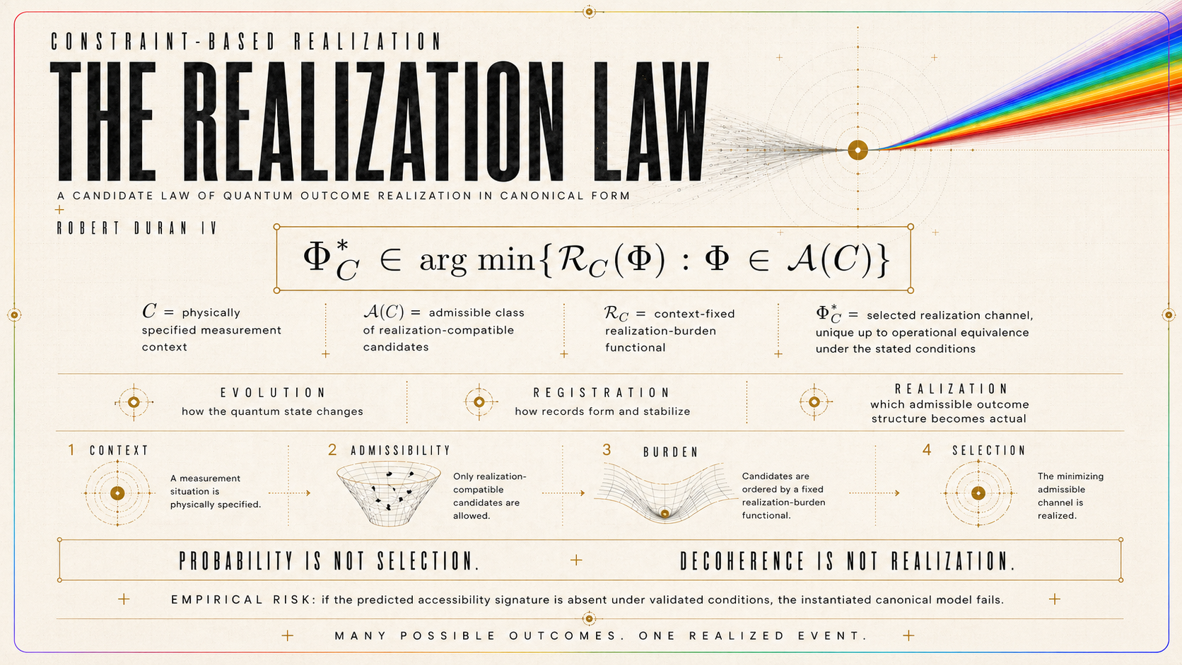
This paper presents Constraint-Based Realization (CBR) in canonical form as a single-outcome realization-law framework intended to compress the theory into an exact mathematical and empirical object. A canonical realization law is defined over a restricted admissible class of realization channels and shown, under the stated admissibility axioms, to be structurally representable rather than freely selected. Under additional regularity conditions, the selected realization channel is unique up to operational equivalence. Within the canonical admissibility structure, the paper further proves a local probability-closure result: admissible refinement, operational invariance, symmetry, normalization, nontriviality, and regularity force quadratic modulus weighting, excluding distinct normalized nonquadratic alternatives.
To render the theory empirically vulnerable, the paper defines an operational accessibility parameter η for record-bearing measurement contexts, identifies a critical accessibility regime η_c, and embeds the theory in a designated delayed-choice record-accessibility protocol family. Relative to a validated standard-quantum baseline comparator, it derives a bounded accessibility-signature regime, a lower-bound deviation structure conditional on nontrivial accessibility relevance, and a detectability theorem for the instantiated canonical response. A bounded nuisance class is then introduced, together with a nuisance-separation theorem and a strong-null failure condition: if validated baseline-class behavior persists across the accessibility-critical regime under the declared detectability conditions, the instantiated canonical model is false.
The paper does not claim universal closure over all realization-law alternatives, final universal Born-neutrality closure across all admissibility geometries, or broad empirical deviation across ordinary measurement settings. Its claim is narrower and more exact. It presents CBR in canonical law form, restricts its admissible realization class, secures restricted uniqueness and local weighting closure within that class, operationalizes accessibility, and places the resulting theory under a finite, public, protocol-specific empirical burden. In that sense, the paper advances CBR from a distributed research architecture to a canonically specified and experimentally vulnerable theory candidate.

1. Introduction
1.1 The unresolved target
The present paper addresses a narrow but foundational question in quantum theory: what, if anything, constitutes the physical law by which one outcome structure is realized in an individual measurement context? This question must be stated exactly. Standard quantum mechanics supplies a highly successful account of state evolution, whether through unitary propagation in closed systems or effective dynamical maps in open systems. It also supports a rich account of correlation, decoherence, environmental entanglement, and instrument-level state updating. What it does not by itself transparently furnish is a law of single realized outcome selection. That is the target of the present work.
Three issues must therefore be distinguished. First, there is the evolution of the quantum state or reduced state under the ordinary dynamical rules of the theory. Second, there is the formation of measurement-correlated records, including pointer-state stabilization, branching structure in decohering descriptions, and effective interference suppression in reduced descriptions. Third, there is the further question of why, in a given physical circumstance, one outcome structure is realized rather than the mere persistence of a formal correlated description across alternatives. The first two are indispensable to any realistic account of measurement. Neither, by itself, settles the third.
This distinction is not semantic. Unitary or open-system evolution specifies how amplitudes, phases, and correlations evolve. Decoherence explains why interference may become effectively inaccessible and why certain record-bearing structures become dynamically stable. Yet decoherence alone does not transparently furnish a physical rule stating why one outcome obtains rather than merely why a reduced subsystem-relative description becomes quasiclassical. Some frameworks interpret that gap away, others absorb it into branching ontology, and others treat it as requiring additional law. The present paper proceeds only from the claim that if one seeks a realization law, then that law must be stated in explicit physical and mathematical form.
Accordingly, this paper does not enter the measurement problem through generalized interpretive discourse. Its concern is not to survey philosophical packages or restate familiar interpretive positions in new language. Its concern is narrower and more demanding. It asks whether outcome realization can be formulated as a constrained law-selection problem, whether that law can be canonically specified rather than ad hoc, and whether it can be rendered vulnerable to empirical failure. Constraint-Based Realization is introduced here not as a generic interpretive stance, but as a candidate realization-law framework whose adequacy depends on formal admissibility, restricted uniqueness, local weighting closure, operational consequence, and public empirical exposure.
1.2 What this paper does
This paper does not widen the CBR program. It fixes its minimal canon. Its task is to state one realization-law object sharply enough that it can be evaluated as a theory candidate rather than as a developing framework. Accordingly, the paper has four exact organizing aims. It fixes a canonical law form, restricts the admissible realization class, defines an operational accessibility variable, and derives a finite empirical burden for the resulting theory. These four aims remain the organizing structure of the paper, but they now culminate in a stronger internal architecture than earlier versions did.
First, the paper canonizes the law form. For each measurement context C, it defines an admissible class 𝒜(C) of realization-compatible channels and a realization functional ℛ_C, with the selected channel Φ*_C chosen as the minimizer of ℛ_C over 𝒜(C). The point of this construction is not maximal generality. It is to eliminate residual plasticity at the level of the realization law itself. A theory candidate cannot remain indefinitely permissive about its central selection rule and still claim formal seriousness.
Second, the paper restricts admissibility. Not every formally definable channel is permitted to count as a realization law. The admissible class is narrowed by excluding channels whose apparent selectivity depends on representational artifacts, arbitrary labeling, accessibility-insensitive degeneracy, or hidden post hoc weighting. Within the theorem class treated here, the canonical law is not left merely stipulated. It is shown to be representable in canonical form under the stated admissibility axioms, and, under additional regularity conditions, the selected realization channel is unique up to operational equivalence. The resulting uniqueness claim is intentionally restricted rather than universal: within the canonical admissibility class, realization is fixed up to operational equivalence and not by descriptive accident.
Third, the paper operationalizes accessibility. If record structure is physically relevant to realization, then accessibility must be defined at the protocol level rather than left as a conceptual placeholder. The paper therefore introduces η as an operational accessibility parameter governing the physically relevant availability of outcome-defining records, with η_c identifying the critical accessibility regime in which accessibility becomes realization-effective. This is the bridge between the formal law and the empirical domain in which the law must either become visible or fail.
Fourth, the paper derives a finite empirical burden. It identifies a canonical protocol family in which accessibility can become realization-relevant in a nontrivial way and proves a restricted accessibility-signature claim for that domain. In the strengthened final form of the paper, this burden is sharper than a generic signature claim. The theory is tied to a bounded accessibility-critical regime, a lower-bound deviation structure, a detectability condition, a nuisance-separation requirement, and a strong-null failure criterion for the instantiated canonical model. The paper therefore does not end with a sharpened interpretation. It ends with a finite experimental liability.
These four aims now operate as a cumulative sequence. Canonical law form without admissibility restriction remains underdetermined. Admissibility restriction without local closure of the associated weighting structure remains probabilistically incomplete. Accessibility without a bounded critical regime remains too loose to bear theorem-level empirical weight. And a signature claim without nuisance separation and a strong-null failure condition remains incomplete as a public test burden. The present paper is constructed to close exactly that sequence and no more.
1.3 What this paper does not claim
The strength of a realization-law proposal depends not only on what it asserts, but on what it refuses to assert without proof. The present paper therefore makes its non-claims explicit and keeps them narrow. Its aim is not to present CBR as a finished universal completion of quantum foundations, but to isolate one canonical law form, one admissibility structure, one operational control variable, and one finite empirical burden. Everything beyond that is either outside the scope of the paper or left deliberately open.
First, this paper does not claim universal closure over all possible realization-law alternatives. The results established here are internal to the canonical CBR form under the stated axioms, regularity assumptions, and protocol conditions. They do not show that every logically conceivable realization-law framework outside this structure is impossible, nor that every rival admissibility architecture has been eliminated in full generality. What is claimed is narrower and stronger: within the declared scope, the canonical CBR law is non-arbitrary, structurally constrained, and sufficiently rigid to incur a genuine empirical burden.
Second, this paper does not claim final universal Born-neutrality closure. What it does now establish is stronger but still local: within canonical admissibility, once admissible refinement, operational invariance, symmetry, normalization, nontriviality, and regularity are fixed, no distinct normalized nonquadratic weighting survives. That is a local probability-closure result inside the canonical theory, not a universal theorem across every conceivable realization framework or admissibility geometry. The deeper global closure burden remains separate. It is not denied, and it is not concealed.
Third, this paper does not claim broad empirical deviation from standard quantum mechanics across ordinary measurement settings. The empirical burden developed here is restricted to a designated accessibility-sensitive protocol family. That restriction is intentional. A law candidate becomes scientifically legible by exposing one finite test domain first, not by claiming ubiquitous visible departure everywhere. The present paper therefore does not argue that every measurement context should exhibit realization-sensitive anomaly. It argues only that if accessibility enters realization law nontrivially, then there must exist a designated protocol regime in which baseline-class global equivalence fails and in which the instantiated canonical model incurs a public failure condition under validated null behavior.
Fourth, this paper does not claim to settle every interpretive question surrounding quantum measurement. It does not attempt to dissolve the problem by metaphysical stipulation, nor does it attempt to refute all alternatives by interpretive comparison alone. Its concern is narrower: whether one can write down a canonically specified realization law, restrict it enough to make it non-arbitrary, connect it to an operational accessibility variable, secure local closure of its internal weighting burden, and state a finite condition under which it would fail. The paper should therefore be read as a law-candidate compression of the CBR program, not as a universal manifesto about all of quantum foundations.
These non-claims do not weaken the present result. They are what keep it scientifically credible. A theory candidate does not become stronger by claiming more than it has earned. It becomes stronger by forcing one exact object into the open, stating what has been fixed, stating what has not been fixed, and exposing the fixed part to failure without pretending that the unfixed part has already been solved. That is the standard this paper adopts.
1.4 Why this paper is necessary
The present paper is necessary because the earlier stages of the CBR program, however substantial, do not by themselves yield a single theorem-bearing object that can be judged as a law candidate in its own right. A research program may contain formal architecture, narrowing arguments, comparative pressure, and empirical ambition while still remaining too distributed to count as one canonically specified theory. That is the gap this paper is written to close. Its necessity lies not in expanding the program, but in compressing it to the point where the central law form, the admissibility structure, the operational control variable, and the empirical failure condition all stand together in one place.
Without that compression, the framework remains vulnerable to a familiar objection: that it may be serious, suggestive, and increasingly disciplined, but still too permissive at the point where a theory must become exact. A realization-law proposal does not become scientifically legible merely by arguing that the measurement problem is real, that accessibility may matter, or that some later experiment might discriminate among completion strategies. It becomes legible when the following are fixed simultaneously: the law form, the admissible class, the representational status of that law, the uniqueness status of the selected channel, the local status of the associated weighting structure, the operational variable through which empirical burden is incurred, and the condition under which failure of the relevant signature counts against the theory itself.
More specifically, the earlier work established four prerequisites that now require compression rather than repetition. It established that realization must be distinguished from ordinary evolution and record registration. It established that admissibility cannot remain indefinite if the framework is to be more than a structured redescription. It established that accessibility, if physically relevant, must become operational rather than merely conceptual. And it established that a law candidate must incur empirical burden rather than remain indefinitely sheltered inside interpretive language. What had not yet been produced was a compact canonical statement in which those burdens are bound together tightly enough that a skeptic can no longer ask what the actual theory is. This paper is that statement.
Its necessity is therefore methodological as much as formal. A theory candidate must eventually move from developmental architecture to canonical exposure. At that point, the relevant question is no longer whether the surrounding program is interesting or ambitious. The relevant question is whether one exact object can be written down such that it is constrained enough to be judged, narrow enough to be challenged, and vulnerable enough to fail. In the strengthened form presented here, that object now includes canonical representation, restricted uniqueness up to operational equivalence, local probability closure within canonical admissibility, operational accessibility, and nuisance-separated empirical exposure. The paper therefore ceases to be merely developmental and becomes a canonically specified, mathematically constrained, and finitely exposed theory candidate.

2. Foundations of the Realization Problem
2.1 Evolution, registration, realization
The formal clarity of the present framework depends on maintaining a strict distinction among three layers of physical description: evolution, registration, and realization. These layers are related, but they are not identical, and a realization-law proposal becomes unstable if they are allowed to collapse into one another.
Evolution denotes the ordinary dynamical behavior of the quantum state or reduced state. In closed settings, this is represented by unitary propagation on a Hilbert space ℋ. In open or instrument-level settings, one may instead use reduced dynamics, effective maps, or CPTP descriptions. The essential point is unchanged: evolution governs how amplitudes, phases, correlations, and entanglement structure change in time under the accepted dynamical rules of the theory. It does not, by that fact alone, specify a law by which one outcome structure is realized.
Registration denotes the physical formation of records. This includes stable pointer-state structure, durable system-apparatus correlation, environmental encoding, and the emergence of record-bearing organization capable of later retrieval or effective classical description. Registration is therefore a genuine physical achievement of a measurement interaction. It is what makes there be something record-like in the world. But even fully developed registration does not yet answer the further question of why one outcome structure is realized in a single case rather than merely represented in a correlated formal description.
Realization, as used in this paper, denotes that further physically selective level. It is not identified with observation, reporting, linguistic declaration, or epistemic update. Nor is it treated as a synonym for decoherence, branching, or the mere existence of system-record correlation. It refers to the law-governed selection of an outcome channel once the admissible structures of evolution and registration are already in place. In the CBR framework, realization is the level at which a law must operate if the measurement problem is to be treated as a problem of outcome selection rather than only as a problem of state description.
This threefold distinction is introduced not to multiply entities unnecessarily, but to prevent equivocation. If evolution is supposed to do all the work, then one must explain how ordinary state propagation alone yields single realized outcomes. If registration is supposed to do all the work, then one must explain why correlation and record formation alone count as selection rather than merely as structure. If neither explanation is accepted as complete, then a distinct realization level becomes unavoidable for the purposes of the present framework. CBR is therefore located explicitly at that third level. It presupposes the ordinary formal apparatus of evolution and the physical relevance of registration, but it does not reduce realization to either of them.
This distinction also fixes the scope of the theory. CBR is not a replacement for quantum dynamics, and it is not a competing theory of decoherence. It is a proposal about what additional law structure is required if one insists that single-outcome realization is a physical question not exhausted by evolution and registration alone. The later sections then impose the additional burdens needed for such a proposal to become serious: admissibility restriction, canonical representation, restricted uniqueness, local weighting closure, operational accessibility, and public empirical exposure.

2.2 Mathematical setting
Let ℋ denote the Hilbert space associated with the total physical degrees of freedom relevant to the measurement context under consideration, and let 𝒟(ℋ) denote the set of density operators on ℋ. A measurement context is denoted by C.
The symbol C is not intended to represent only an observable label or a basis choice. It denotes the physically specified measurement arrangement insofar as that arrangement is relevant to realization. In particular, C may include instrument structure, interaction architecture, record-bearing degrees of freedom, timing relations relevant to registration and retrieval, and the accessibility properties of any outcome-defining information carriers.
The theory therefore begins from physically specified contexts, not from abstract observables alone.
For each physically well-defined context C, assume there exists a nonempty admissible class 𝒜(C) of realization-compatible channels. Each Φ ∈ 𝒜(C) is a candidate realization channel: a formally and physically permissible outcome-selection structure relative to the context. Admissibility is not equated with arbitrary formal constructibility.
The class 𝒜(C) is restricted by physical criteria developed later in the paper, including non-arbitrariness, representational invariance, record-structural relevance, accessibility consistency, admissibility separation, and local weighting neutrality. Thus 𝒜(C) is not the set of all mathematically writable maps on 𝒟(ℋ), but the set of candidate realization channels surviving the canonical physical constraints.
A realization functional ℛ_C is then defined on 𝒜(C), with codomain in ℝ or an ordered subset sufficient to support comparison and minimization. Its role is to assign to each admissible candidate channel Φ a realization burden measuring the extent to which that channel satisfies or violates the canonical constraints of the framework.
The selected realization channel Φ_C is chosen as the minimizer of ℛ_C over 𝒜(C). Equivalently, Φ_C is the admissible channel that minimizes the realization burden in context C.
This is the schematic heart of canonical CBR. It states that realization, within a physically specified context, is selected not by arbitrary labeling, stipulation, or concealed reintroduction of target weights, but by constrained minimization over a physically admissible class. The minimization need not be interpreted as naive energetic minimization or as variational dynamics in the ordinary sense.
Its meaning is narrower and exact: realization is fixed by the most constraint-satisfying admissible channel once the context is given.
Three clarifications are required.
First, Φ*_C need not be unique in the strict syntactic sense. What matters physically is uniqueness up to operational equivalence. If two candidate channels differ only by representational structure that leaves all physically relevant observables and accessibility relations unchanged, they belong to the same operational verdict class. The uniqueness sought in this paper is therefore restricted uniqueness modulo operational equivalence, not absolute formal uniqueness under every conceivable redescription.
Second, the use of channel language does not commit the framework to an ordinary instrument reading of realization. The channel formalism is adopted because it provides the cleanest canonical vehicle for stating admissibility, equivalence, minimization, and operational consequence in a mathematically disciplined way. Whether every physically relevant feature of realization can be encoded in standard CPTP language without extension is a further technical question, not a presupposition of the present paper.
Third, accessibility will become essential. Not every record is physically relevant in the same way, and not every formal correlation should count equally in realization judgment. For that reason, the context is not exhausted by bare system-apparatus observable structure. It includes, in a physically significant way, the conditions under which outcome-defining information is stored, retrievable, stable, and available to further physical interaction.
This motivates the later introduction of the operational accessibility parameter η and the corresponding accessibility-sensitive distinctions within 𝒜(C).
The mathematical setting is therefore deliberately modest and deliberately sharp. It assumes only what is needed to turn the realization question into a law-selection problem with explicit formal objects: a state space ℋ, a density-operator space 𝒟(ℋ), a physically specified context C, a constrained admissible class 𝒜(C), a realization functional ℛ_C, and a selected channel Φ*_C defined by constrained minimization.
2.3 The formal question
With the foregoing distinctions and notation in place, the central formal question of the paper can be stated exactly:
Given a measurement context C, what physical law selects the realized outcome channel Φ*_C from the admissible class 𝒜(C)?
This formulation is more precise than the generic question of how “collapse” occurs and more disciplined than the request for an “interpretation of measurement.” It presupposes that the relevant problem is not merely to describe the evolution of amplitudes, nor merely to note the existence of correlated records, but to identify the law by which one realization-compatible channel is selected from among those channels that remain physically admissible in the given context.
Several features of this formulation deserve emphasis.
First, the question is context-indexed. There is no presumption here that realization law can be stated independently of physical measurement architecture, record structure, timing relations, or accessibility conditions. Context dependence is not treated as a defect. It is treated as the natural form of any law whose function is to connect outcome selection to physically meaningful constraints. At the same time, context-indexing must not collapse into arbitrariness.
The law must remain invariant under physically irrelevant reformulations and must preserve operational equivalence across equivalent realizations of the same physical situation.
Second, the question is selective rather than merely descriptive. It does not ask how one may redescribe a measurement after the fact, nor how one updates a state assignment upon learning an outcome. It asks what channel is selected, by what law, prior to any merely epistemic reinterpretation. In that sense, the law sought here is physically selective even if its formal expression is operational.
Third, the question is canonically constraining. The paper is not satisfied with any selection rule that reproduces the desired verdict by hidden stipulation. It seeks a law form narrow enough to exclude arbitrary selectivity, a class of admissible channels disciplined enough to support canonical representation and restricted uniqueness, and a weighting structure locally constrained enough that probability is not left as a free internal design choice.
Fourth, the question is empirically exposed. The theory cannot remain satisfied with a formal selection rule alone. If accessibility is physically relevant to realization, then the law must eventually identify an operational variable, a designated protocol family, a bounded critical regime, a detectability condition, and a public failure criterion. The task of the remainder of the paper is to show that these requirements can be made exact in canonical CBR.
3. Axioms of Canonical CBR
The present section states the minimal axiom set under which CBR is to be read as a canonical realization-law proposal rather than as a suggestive framework. The purpose of these axioms is not to maximize generality. It is to minimize arbitrariness. A realization theory that leaves its admissible structures indefinite, its selection rule plastic, its weighting burden unconstrained, or its empirical standing optional does not yet count as a serious law candidate.
These axioms are therefore not presented as metaphysical slogans. They are the canonical constraints that make later representation, restricted uniqueness, local probability closure, and empirical exposure possible. They do not, by themselves, prove the later theorems. But they fix the theory’s admissible starting point and exclude the most immediate forms of hidden arbitrariness. In that sense, they should be read not as decorative commitments, but as the minimal conditions under which the later sections can ask a well-posed question.

3.1 Axiom A1 — Dynamical compatibility
Axiom A1. The realization law must not replace or covertly modify the ordinary quantum dynamics that govern the evolution of the underlying state description outside realization selection.
The purpose of A1 is to keep the target of the theory narrow. CBR is not introduced as a replacement for standard quantum evolution, nor as an unrestricted dynamical revision of the theory’s propagation rules. Its task is to specify a law of realization once the relevant dynamical and registration structure is already in place. If the realization law were allowed to absorb or secretly alter the ordinary evolution, then the theory would become ambiguous at the level of target: it would no longer be clear whether CBR is a realization law, a collapse dynamics, or a wholesale substitute for standard evolution.
A1 therefore preserves the architecture established in Section 2. Evolution remains evolution. Registration remains registration. Realization is introduced as an additional law-bearing layer rather than as a disguised modification of the underlying dynamics. This axiom does not forbid that realization may have empirically distinct consequences in designated regimes. It forbids only the blurring of realization into a covert rewrite of the baseline dynamical theory.
3.2 Axiom A2 — Context-indexed admissibility
Axiom A2. For each physically specified measurement context C, there exists a nonempty admissible class 𝒜(C) of realization-compatible channels over which realization selection is defined.
A2 formalizes the context-indexed character of the theory. Realization is not treated as a context-free verdict imposed on an abstract state independently of measurement architecture, record structure, timing, or accessibility conditions. It is treated as a law selecting from an admissible class relative to a physically specified context.
The point of this axiom is twofold. First, it excludes the idea that realization selection can remain indefinitely vague while still claiming formal status. If there is no admissible class, there is no object for the law to select over. Second, it avoids the opposite mistake of permitting every formally writable channel to count as a candidate realization rule. The admissible class must be nonempty, but it must also be physically restricted. This is what makes later sections meaningful. Canonical representation, restricted uniqueness, and local weighting closure all presuppose that realization is posed over a genuine admissible class rather than an unbounded space of formal possibilities.
A2 is therefore the axiom that turns the realization problem from an interpretive slogan into a constrained selection problem.
3.3 Axiom A3 — Representational invariance
Axiom A3. Realization selection must be invariant under physically irrelevant reformulations of the same context, including relabelings, equivalent encodings, and descriptively different but operationally indistinguishable representations.
The rationale for A3 is straightforward. A realization law that changes its verdict under purely formal redescription is not physically selecting; it is responding to notation. If two channel descriptions differ only by representational form while preserving all realization-relevant physical content, then the law must treat them equivalently.
This axiom is essential to the later canonical representation theorem. Without representational invariance, one cannot separate the physically meaningful content of the law from arbitrary descriptive packaging. Nor can one later state restricted uniqueness up to operational equivalence in a clean way. A3 therefore protects the theory from one of the most common pathologies of underconstrained formal proposals: the appearance of law-level structure that is actually an artifact of representation.
In practical terms, A3 means that the theory cannot manufacture selectivity by hidden relabeling, hidden channel reparameterization, or equivalent contextual recodings. If realization is physical, it must remain stable under physically irrelevant reformulation.
3.4 Axiom A4 — Record-structural relevance
Axiom A4. Realization selection may depend only on physically relevant record structure present in the context and not on abstract branch descriptions lacking record-bearing significance.
This axiom follows from the distinction between correlation and realization. Not every formal decomposition of the state carries the same physical significance. A4 requires that realization be sensitive only to structures that genuinely participate in the record-bearing organization of the context.
The point is not to say that realization is identical to record formation. It is not. Rather, the point is that realization cannot be allowed to depend on purely formal branch distinctions that fail to correspond to physically operative record structures. Without A4, the theory could drift into arbitrary fine-graining or syntactic channel distinctions that have no measurement-level relevance.
A4 is therefore one of the key constraints preventing CBR from becoming a branch-labeling exercise. It insists that the admissible realization problem be anchored in the physically relevant architecture of record-bearing contexts rather than in formal decomposition alone.
3.5 Axiom A5 — Accessibility relevance
Axiom A5. If record structure is physically relevant to realization, then the realization law may depend nontrivially on the operational accessibility of that record structure.
A5 introduces the key bridge to the later empirical burden. It does not yet define accessibility. That task belongs later. What it does is state that if records matter to realization, then it is not enough for them merely to exist as formal correlations. Their physically operative availability may also matter.
This axiom is necessary because the theory aims to distinguish among several nonequivalent cases: a merely formal correlation, a fragile record that cannot be stably recovered, and a durable operationally available record. If realization were indifferent to those differences, then accessibility would drop out of the theory and the designated protocol family would lose its point. If accessibility is relevant, however, that relevance must later be operationalized through η and tied to a bounded empirical burden.
A5 therefore does not yet prove anything empirical. It states the structural opening through which accessibility becomes law-level relevant.
3.6 Axiom A6 — Probabilistic non-insertion
Axiom A6. The canonical realization law must not secure its probabilistic structure by covert definitional insertion of the target weighting rule.
This axiom should be read with precision. It does not say that the present paper already proves final universal probabilistic closure at the axiom stage. It says that the law may not simply assume, hide, or redefine the target weighting structure inside its admissibility metric, burden geometry, refinement rules, or normalization conventions and then present the resulting output as if it were derived.
A6 is therefore a prohibition against probabilistic circularity at the canonical starting point. The later probabilistic theorem does more than earlier versions of the paper did: it proves a local probability-closure result within canonical admissibility, showing that no distinct normalized nonquadratic weighting survives once admissible refinement, operational invariance, symmetry, normalization, nontriviality, and regularity are fixed. But that later result is only meaningful if the axiomatic starting point has already ruled out covert insertion. A6 is what secures that discipline.
In other words, A6 does not itself deliver the local closure theorem. It makes that theorem worth having.
3.7 Axiom A7 — Empirical exposure
Axiom A7. A canonical realization law must incur a finite empirical burden in a designated protocol family and must admit a public condition under which the instantiated theory fails.
A7 is the final axiom because it prevents the framework from remaining indefinitely interpretive. A realization-law proposal becomes scientifically serious only when it does not merely say how one could think about outcome selection, but also says where that law becomes empirically vulnerable.
In the stronger final architecture of the paper, this axiom has sharper consequences than before. It is no longer satisfied merely by saying that some generic accessibility-sensitive signature might occur in principle. It is satisfied only when the law is tied to an operational accessibility variable, a designated protocol family, a bounded accessibility-critical regime, a lower-bound deviation structure, a detectability condition, a nuisance-separation theorem, and a strong-null failure criterion for the instantiated canonical model.
A7 therefore states the paper’s public standard. The law must not only be canonically specified. It must be finitely exposed.
3.8 What the axiom set accomplishes
Taken together, A1 through A7 do not yet prove the main theorems of the paper. They do something prior and necessary. They specify the minimal canonical conditions under which CBR can count as a realization-law proposal at all.
A1 fixes the narrow target by preserving ordinary dynamics outside realization selection.
A2 turns realization into a context-indexed admissible selection problem.
A3 excludes representational arbitrariness.
A4 anchors realization in physically relevant record structure.
A5 opens the law to operational accessibility where that relevance is genuine.
A6 forbids covert probabilistic insertion and prepares the ground for later local probability closure.
A7 prevents the theory from retreating into optional empiricism by requiring finite exposure and a public failure condition.
The consequence is that the later sections no longer begin from a vague interpretive framework. They begin from a canonically disciplined object: one narrow enough to support representation, restricted uniqueness, local weighting closure, operational parameterization, and bounded empirical burden. That is exactly what this axiom set is meant to achieve.
4. Canonical Law Form
The axiom set of the previous section fixes the constraints under which a realization-law proposal may count as physically serious. The present section states the corresponding law form. Its task is not to introduce one useful selection functional among many. Its task is to identify the minimal burden structure capable of satisfying the axioms without collapsing into arbitrariness, hidden probabilistic insertion, or empirical idleness. The claim of canonicality made here is therefore restricted but exact. It is not the claim that no other realization-law theory could ever be written. It is the claim that, within the stated axioms and within the scope of the present paper, the law form has been compressed to the point where its surviving structure is no longer optional.
The section has four parts. First, it defines the realization functional. Second, it specifies the selected realization rule. Third, it explains why the resulting form is canonical rather than merely convenient. Fourth, it clarifies the exact sense in which canonicality is being claimed. The point of the section is to make the law feel mathematically and physically necessary within scope, not merely elegant.
4.1 Definition of the realization functional
Let C be a physically specified measurement context and let 𝒜(C) denote the corresponding admissible class of realization-compatible channels. The realization functional is defined on 𝒜(C) by
ℛ_C(Φ) = α Ξ_C(Φ) + β Ω_C(Φ) + γ Λ_C(Φ),
where α, β, γ ≥ 0 are fixed theory-level coefficients and where each term measures a distinct burden that a candidate realization channel must bear if it is to count as canonically admissible.
The first term, Ξ_C(Φ), is the representational invariance burden. It measures the extent to which the realization verdict induced by Φ fails to remain stable under physically irrelevant reformulations of the context. A channel carries low Ξ_C burden only if its realization effect is invariant under relabeling, equivalent encoding, coordinate change, basis redescription, or other descriptive transformations that leave the realization-relevant physical content unchanged. This term is forced by A3. A realization law that depends on notation is not a realization law at all.
The second term, Ω_C(Φ), is the record-structural coherence burden. It measures the extent to which Φ fails to align realization selection with the actual record-bearing structure of the context. A channel carries low Ω_C burden only if it tracks physically meaningful record organization rather than unsupported formal branch multiplicity or mathematically available but operationally idle distinctions. This term is forced by A4. A realization law that does not distinguish genuine record structure from formal surplus cannot claim physical selectivity.
The third term, Λ_C(Φ), is the accessibility-consistency burden. It measures the extent to which Φ fails to respond coherently to the operational accessibility structure of the context. A channel carries low Λ_C burden only if it treats accessibility-equivalent contexts equivalently and permits accessibility, when physically relevant, to enter the law through operationally meaningful distinctions rather than through undeclared implementation noise. This term is forced by A5 and A7. Without it, accessibility can be named but not lawfully integrated.
The coefficients α, β, and γ are not protocol-level fitting knobs. They belong to the law form itself. Their role is to fix the comparative weight of the three irreducible burden classes at the level of the canonical theory. Up to overall positive rescaling, what matters is their relative structure rather than arbitrary normalization. A theory that adjusted these coefficients opportunistically from one context to the next would not possess a canonical realization law. It would possess only a family of loosely related selection heuristics.
The present decomposition is deliberately minimal. It contains no separate probability-matching term, because such a term would violate or at least endanger the restricted Born-neutrality discipline of A6 unless independently forced. It contains no separate branch-count penalty, because unsupported multiplicity is already penalized insofar as it produces record-incoherent realization structure and therefore contributes to Ω_C. It contains no independent gauge-fixing penalty, because descriptive arbitrariness is already captured by Ξ_C. The three-term form is therefore not intended as one elegant functional among many equally good alternatives. It is intended as the smallest burden decomposition sufficient to carry the exact axiomatic load of the paper.
4.2 Canonical selection rule
With the realization functional defined, the selected realization channel is given by
Φ*_C = argmin{ℛ_C(Φ) : Φ ∈ 𝒜(C)}
This is the canonical selection rule of the theory.
Its meaning should be stated carefully. The rule does not say that realization is chosen by arbitrary optimization over every formally writable map. It says that, once the physically admissible class has been restricted by the axioms, the realized channel is the admissible channel that minimizes the total realization burden. The minimization is therefore constrained twice: first by admissibility, and second by the burden structure. This is essential. Without admissibility, minimization would range over a space too broad to support any meaningful uniqueness claim. Without the burden functional, admissibility would remain a mere negative filter and would not yet yield selection.
The selected channel need not be unique in the strict syntactic sense. What matters physically is uniqueness up to operational equivalence. If two admissible channels differ only by representational structure that leaves all realization-relevant observables, record relations, and accessibility consequences unchanged, then they belong to the same selected verdict class. The law therefore selects a realization class modulo operationally null reformulation, not necessarily a single formula under every possible redescription.
This rule is also not to be confused with ordinary energetic or variational minimization in mechanics. The functional ℛ_C does not measure energy, action, or entropy in the conventional sense unless some future specialization supplies such an interpretation. Its role here is narrower. It measures the total law-burden carried by a candidate realization channel relative to the axiomatic constraints of the theory. The selected channel is therefore the least arbitrary, most record-coherent, and most accessibility-consistent admissible realization structure available in the context.
4.3 Why this is the canonical form
The claim that ℛ_C is canonical must be justified with precision. In the present paper, canonicality does not mean metaphysical inevitability across every imaginable realization-law theory. It means something narrower and stronger within scope: given A1–A7, no retained burden term is dispensable, and no omitted burden term is independently required to make the law physically serious. Canonicality is therefore a claim of minimal sufficiency under constraint, not of universal finality across all logically possible alternatives.
The first reason this form is canonical is that each retained term is axiom-forced. Without Ξ_C, the theory cannot exclude realization verdicts that change under physically irrelevant reformulation and therefore fails the non-arbitrariness demand of A3. Without Ω_C, the theory loses its anchoring in the actual record-bearing structure of the context and cannot satisfy A4. Without Λ_C, accessibility can be named but not integrated into the realization law, and the theory loses both its operational content and its route to empirical exposure under A5 and A7. The retained terms are therefore not stylistic choices. They are the minimal burden coordinates required by the axioms themselves.
The second reason this form is canonical is that the main omitted alternatives are either redundant, illicit, or empirically idle. A separate term rewarding preferred basis choice without additional physical content would merely duplicate representational dependence already penalized by Ξ_C. A separate term penalizing unsupported branch multiplicity would add no indispensable burden not already captured by Ω_C, provided record-structural coherence is defined correctly. A separate empirical-fit term designed to reward agreement with future data would violate the logic of the paper by inserting success criteria directly into the law. A direct probability-insertion term would violate A6 unless independently derived from the admissibility structure itself. Thus the omitted candidates are not absent through oversight. They are absent because the exact work they might appear to do is either already done by the canonical burdens or else would deform the theory into something less disciplined.
The third reason this form is canonical is that it is already sufficient to support the full theorem program of the paper. The realization functional, as defined, is strong enough to support restricted uniqueness, strong enough to make accessibility operationally relevant, and strong enough to incur a finite empirical burden in the designated protocol family. A richer functional may be conceivable, but richness alone is not a virtue at this stage. Unless additional structure is forced by theorem or experiment, added burden terms would increase descriptive surface without increasing explanatory necessity. The correct canonical form is therefore the smallest one that can already bear the full load of law selection, admissibility restriction, and empirical exposure.
Canonicality in this sense is not ornamental language. It is the statement that, within the declared scope of the paper, the law has been compressed until its surviving structure is no longer optional. That is what distinguishes a canonically specified realization functional from a merely well-designed heuristic.
4.4 Restricted sense of canonicality
The paper’s claim of canonicality is deliberately restricted, and that restriction should be stated explicitly.
First, the paper does not claim that the present three-term decomposition is the unique formally conceivable realization functional in all of logic. It claims only that within the axiomatically constrained class relevant to canonical CBR, the retained structure is minimal and sufficient.
Second, the paper does not claim that every future implementation or extension must preserve the exact same microscopic interpretation of Ξ_C, Ω_C, and Λ_C in every context. What is fixed here is the canonical burden architecture, not every later platform-specific realization of that architecture.
Third, the paper does not claim that no future stronger theorem could further constrain the functional. On the contrary, one natural future development would be a restricted representation theorem showing that any realization functional satisfying the same admissibility, invariance, record, accessibility, and empirical-accountability constraints is equivalent to the present one up to positive affine rescaling and operationally null structure. The present paper stops short of that stronger claim.
These restrictions do not weaken the section. They define its exact success condition. The present result is that canonical CBR now possesses a law form narrow enough to support theorem-bearing selection and empirical consequence without pretending to have solved every possible problem of generality at once.
4.5 What this section accomplishes
With the realization functional and the canonical selection rule now fixed, the theory has crossed an important threshold. Before this section, the paper had an axiomatic demand for a constrained realization law. After this section, it has a definite law form whose surviving burden terms are justified by the axioms and whose selected channel is defined by constrained minimization over an admissible class.
That is the minimum formal threshold a realization-law proposal must cross before questions of uniqueness, accessibility, empirical signature, and failure can even be asked in exact form. The next section takes the first of those questions directly: whether the canonical law, once posed on its admissible class, actually selects a unique realization class up to operational equivalence.
5. Admissibility, Canonical Representation, and Restricted Uniqueness
5.1 Scope and objective
The canonical law form introduced above is only scientifically meaningful if it is more than a convenient parametrization. The next burden is therefore not merely to state a law, but to show that, once admissibility is constrained by physical and operational consistency, the law is forced into a canonical representation class rather than selected from among equally viable alternatives. This section addresses that burden.
The objective is threefold. First, we formalize the admissibility structure required of any realization law compatible with the conceptual target of CBR. Second, we show that this admissibility structure induces an ordered selection problem representable by a nonnegative burden functional defined on admissible realization channels. Third, under additional regularity and separation assumptions, we establish restricted uniqueness of the realized channel up to operational equivalence.
Throughout, ℋ denotes a finite-dimensional Hilbert space, 𝒟(ℋ) the set of density operators on ℋ, and Ctx the class of admissible experimental contexts. For each context C ∈ Ctx, let 𝒜(C) denote the admissible class of realization channels associated with C. Each Φ ∈ 𝒜(C) is taken to be completely positive and trace-preserving on the context-relevant state space.
A realization law is a map
ℛ : C ↦ Φ*_C ∈ 𝒜(C),
assigning to each admissible context a selected realized channel. The burden of this section is to show that, under the admissibility constraints below, such a law is representable in canonical CBR form and is unique up to operational equivalence under stated conditions.
5.2 Admissibility axioms
We begin by isolating the constraints that any physically acceptable realization law must satisfy.
Axiom 5.1 (Operational well-definedness). If two contexts C and C′ are operationally equivalent, then their admissible channel classes are equivalent under the induced operational identification, and the realization law selects operationally equivalent channels in the two contexts.
This excludes dependence on descriptive presentation rather than physical content.
Axiom 5.2 (Non-vacuity). For every admissible context C, the class 𝒜(C) is nonempty.
This ensures that realization selection is posed over a physically meaningful candidate class.
Axiom 5.3 (Coarse-graining consistency). If C′ is a coarse-graining of C, then the selected channel in C induces, under the canonical coarse-graining map, an admissible selected channel in C′.
This forbids selection rules whose outputs fail to survive observational collapse of description.
Axiom 5.4 (Refinement stability). If C′ is a refinement of C, then the selected channel in C must be recoverable as the induced effective channel of the selected channel in C′.
This prevents realization from depending on arbitrary descriptive resolution.
Axiom 5.5 (Compositional consistency). For independent subcontexts C₁ and C₂, the realization law on the composite context C₁ ⊗ C₂ must be compatible with the channels induced on each factor and with the corresponding factorwise admissibility structure.
This excludes laws whose output depends on whether independent systems are described jointly or separately.
Axiom 5.6 (Label invariance). The realization law may not depend on formal relabelings of outcomes, branches, or auxiliary descriptive coordinates with no operational content.
This removes purely notational or representational arbitrariness.
Axiom 5.7 (Admissibility separation). If Φ, Ψ ∈ 𝒜(C) are not operationally equivalent, then the admissibility structure must preserve their non-equivalence at the level relevant to realization selection.
This excludes pathological admissibility classes in which distinct candidate realizations collapse prematurely into a single indistinguishable selection object.
Axiom 5.8 (Burden monotonicity). If Φ is strictly less admissible than Ψ in context C, in the sense that Φ violates more or stronger admissibility constraints than Ψ, then Φ may not be preferred to Ψ by the realization law.
This converts admissibility from a binary filter into an ordered selection structure.
Axiom 5.9 (Minimal admissibility burden). The realized channel in context C is selected as one of minimal admissibility burden within 𝒜(C), where admissibility burden vanishes only on the realized equivalence class or on a class operationally indistinguishable from it.
Axiom 5.9 should not be read as an aesthetic preference for variational language. Rather, once admissibility induces a stable order of exclusion and residual permissibility, realization selection requires a representation of that order if it is to remain coherent across refinement, coarse-graining, and composition.
5.3 Definitions
We now formalize the admissibility objects used in the theorem sequence.
Definition 5.1 (Operational equivalence). Two channels Φ, Ψ ∈ 𝒜(C) are operationally equivalent, written
Φ ∼ₒₚ Ψ,
if no admissible experiment within context C distinguishes them at the level relevant to realization selection.
Definition 5.2 (Admissibility quotient class). The operational equivalence class of Φ is denoted [Φ]. The quotient space
𝒜(C)/∼ₒₚ
is the space of admissibility-relevant realization classes in context C.
Definition 5.3 (Admissibility preorder). For Φ, Ψ ∈ 𝒜(C), write
Φ ≤_C Ψ
if Φ is no less admissible than Ψ according to the admissibility constraints induced by Axioms 5.1–5.8.
Definition 5.4 (Admissibility burden). An admissibility burden on 𝒜(C) is a functional
B_C : 𝒜(C) → ℝ≥0
such that lower values correspond to greater compatibility with the admissibility structure of the context.
Definition 5.5 (Canonical realization law). A realization law is canonical if for every context C it selects a channel Φ*_C satisfying
Φ*_C ∈ argmin{B_C(Φ) : Φ ∈ 𝒜(C)},
for some admissibility burden B_C invariant under operational equivalence and compatible with refinement, coarse-graining, and composition.
The purpose of the next lemmas is to show that these definitions are not merely formal packaging. They arise because violations of the admissibility axioms generate structural inconsistency.
5.4 Obstruction lemmas
Lemma 5.1 (Equivalence descent). Under Axioms 5.1 and 5.6, the realization law descends to a well-defined map on the quotient space 𝒜(C)/∼ₒₚ.
Proof sketch. Operational well-definedness identifies contexts that differ only by admissibly irrelevant presentation, while label invariance removes dependence on nonphysical coordinates within a fixed presentation. Therefore any two channels lying in the same operational equivalence class must be treated identically by the realization law. Hence realization selection is well-defined on equivalence classes rather than on arbitrary representatives.
Lemma 5.2 (Coarse-graining obstruction). Any realization law violating Axiom 5.3 produces context-dependent inconsistency under observational coarse-graining.
Proof sketch. Suppose a selected channel in a refined context fails to induce an admissible selected image under coarse-graining. Then two experimentally indistinguishable coarse descriptions of the same realized situation will either inherit incompatible selected channels or fail to inherit one at all. This contradicts operational well-definedness.
Lemma 5.3 (Refinement obstruction). Any realization law violating Axiom 5.4 is unstable under admissible refinement and therefore depends on representation rather than physical structure.
Proof sketch. If refinement changes realization selection without an induced recovery of the coarser selected structure, then equivalent physical scenarios described at different resolutions yield different realized outputs. Such dependence is descriptive rather than physical.
Lemma 5.4 (Compositional obstruction). Any realization law violating Axiom 5.5 yields factorization-sensitive realized structure across independent subcontexts.
Proof sketch. Independence requires compatibility between joint description and factorwise description. If realization selection depends on whether independent subsystems are treated jointly or separately, then the law is not physically compositional.
Lemma 5.5 (Admissibility non-collapse). Under Axiom 5.7, inequivalent admissible channels remain distinguishable at the level relevant to selection, and admissibility does not collapse non-equivalent candidates into a trivial selection class.
Proof sketch. If inequivalent channels were admissibly indistinguishable without operational equivalence, then the selection problem would lose the ability to discriminate structurally distinct candidate realizations. This would undermine the meaning of restricted uniqueness.
These lemmas establish that the admissibility axioms are not optional refinements. Their violation produces genuine instability, inconsistency, or trivialization.
5.5 Burden representation of admissibility order
We now show that admissibility induces a representable order structure.
The admissibility preorder ≤_C is defined on the quotient 𝒜(C)/∼ₒₚ by the relative compatibility of admissible realization classes with Axioms 5.1–5.8. Since realization is required to respect that order by Axiom 5.8, the question is whether the preorder admits a scalar representation adequate for canonical selection.
Proposition 5.1 (Order representability). Assume Axioms 5.1–5.8. Then for each context C, the admissibility preorder on 𝒜(C)/∼ₒₚ admits a nonnegative scalar representation by a burden functional B_C, unique up to strictly increasing reparameterization.
Proof sketch. By Lemma 5.1 the relevant selection domain is the quotient by operational equivalence. By Axioms 5.2 and 5.7 this quotient is nonempty and nontrivial. Axioms 5.3–5.5 guarantee that the preorder is stable under the admissibility-preserving maps induced by coarse-graining, refinement, and composition. Axiom 5.8 supplies monotone compatibility between the preorder and realization preference. On a finite or suitably regular quotient class, these properties are sufficient to represent admissibility order by a nonnegative scalar burden functional unique up to order-preserving reparameterization.
The significance of Proposition 5.1 is decisive. Once admissibility induces a stable order, minimization is no longer a stylistic choice. It is the natural representation of admissibility preference.
5.6 Canonical representation theorem
The previous proposition yields a variational representation, but not yet a canonical one. To force canonical CBR form, one must show that admissibility compatibility restricts the burden functional itself.
Let B_can(C) denote the class of burden functionals on 𝒜(C) that are constant on operational equivalence classes and compatible with coarse-graining consistency, refinement stability, compositional consistency, and label invariance.
Proposition 5.2 (Restricted canonicality). Suppose B_C represents the admissibility preorder on 𝒜(C)/∼ₒₚ and is compatible with Axioms 5.1 and 5.3–5.6. Then B_C belongs to B_can(C) up to positive affine renormalization.
Proof sketch. Compatibility with operational well-definedness and label invariance requires B_C to be constant on operational equivalence classes and insensitive to descriptive relabeling. Coarse-graining consistency and refinement stability constrain how B_C transforms across admissibility-preserving maps, excluding burdens that depend on arbitrary descriptive resolution. Compositional consistency excludes context-sensitive cross-terms that do not respect the product structure of independent subcontexts. The surviving class is therefore restricted to burdens equivalent up to positive affine renormalization.
We can now state the main result of the section.
Theorem 5.1 (Canonical representation theorem). Let ℛ be any realization law satisfying Axioms 5.1–5.9. Then for each admissible context C, ℛ is representable, up to operational equivalence and positive affine renormalization of burden, as a canonical CBR selection law of the form
Φ*_C ∈ argmin{B^CBR_C(Φ) : Φ ∈ 𝒜(C)}.
Proof. By Proposition 5.1, the admissibility preorder on the quotient 𝒜(C)/∼ₒₚ admits a nonnegative scalar representation by a burden functional. By Proposition 5.2, any such burden compatible with the admissibility structure belongs to the canonical burden class up to positive affine renormalization. Axiom 5.9 then forces realization selection to occur at a burden minimum. Hence the realization law is representable in canonical CBR form, up to operational equivalence and burden renormalization.
Corollary 5.1 (Structural inevitability of canonical form). Within the admissibility class defined by Axioms 5.1–5.9, canonical CBR form is not an arbitrary proposal but the unique structural representation of admissible realization selection, up to operational equivalence and positive affine renormalization.
This is the core theoretical upgrade. The law no longer appears merely elegant. It appears forced by admissibility structure.
5.7 Restricted uniqueness of the realized channel
Canonical representation is not yet strict uniqueness. That stronger claim requires additional regularity assumptions and should be stated separately.
We therefore introduce the following contextwise regularity conditions.
Assumption 5.R1 (Attainment). For each admissible context C, the admissibility burden B^CBR_C attains its minimum on 𝒜(C).
Assumption 5.R2 (No flat inequivalent degeneracy). There is no burden plateau consisting of multiple inequivalent admissible channel classes all realizing the same minimal burden unless those classes are operationally equivalent.
Assumption 5.R3 (Strict separation). If two admissible channel classes are not operationally equivalent, then the admissibility structure distinguishes them strongly enough to prevent unresolved minimal-burden collapse.
These assumptions are not part of the canonical representation theorem itself. They are additional hypotheses required to convert representability into restricted uniqueness.
Theorem 5.2 (Restricted uniqueness theorem). Assume Axioms 5.1–5.9 and Assumptions 5.R1–5.R3. Then for each admissible context C, the selected realization channel is unique up to operational equivalence.
Proof sketch. By Assumption 5.R1, a minimal-burden admissible channel exists. Suppose there were two inequivalent minimal-burden channel classes. Then either they lie on a flat unresolved burden plateau, contradicting Assumption 5.R2, or the admissibility structure fails to separate inequivalent minima strongly enough for unique selection, contradicting Assumption 5.R3. Hence all minimal-burden channels lie in a single operational equivalence class. By Lemma 5.1, realization selection is therefore unique up to operational equivalence.
Corollary 5.2 (Operational uniqueness). Under Axioms 5.1–5.9 and Assumptions 5.R1–5.R3, realized outcome selection is unique at the operational level.
This is the strongest uniqueness claim warranted at the present stage. It is intentionally restricted. The theorem does not claim strict representative-level uniqueness beyond operational equivalence.
5.8 Consequences for the status of the law
The results of this section materially strengthen the status of canonical CBR. The law is no longer introduced merely as a candidate mathematical form for realization selection. Under the admissibility axioms, it becomes the representational form forced by stable realization ordering. Under the added regularity and separation assumptions, realized selection is unique up to operational equivalence.
This matters because the principal weakness of a newly proposed realization law is often not logical inconsistency but underdetermination: the suspicion that many equally acceptable alternatives remain and that the chosen law is therefore a matter of design rather than necessity. Theorem 5.1 addresses that burden by collapsing admissible realization selection into canonical CBR form. Theorem 5.2 then sharpens that result into restricted uniqueness.
Accordingly, the role of the next section is no longer to justify whether a realization law exists at all, but to determine whether the induced weighting structure is likewise forced rather than selected.
5.9 What this section proves and does not prove
This section proves three things.
First, once admissibility is constrained by operational equivalence, refinement stability, coarse-graining consistency, compositional consistency, label invariance, and admissibility monotonicity, realization selection admits a burden representation.
Second, once that burden representation is required to remain compatible with the same admissibility structure, it collapses into canonical CBR form up to operational equivalence and positive affine renormalization.
Third, under explicit attainment, nondegeneracy, and separation assumptions, the selected realized channel is unique up to operational equivalence.
This section does not prove the strongest imaginable global claim that every conceivable realization law in every mathematical setting must reduce to canonical CBR form. Nor does it establish representative-level uniqueness beyond operational equivalence without additional structural assumptions. Those stronger claims would require broader generality, possibly infinite-dimensional extension, and sharper control of admissibility geometry.
What this section does establish is the claim required for the present program: canonical CBR is not merely a convenient realization law. It is the structurally forced representative of admissible realization selection in the class of contexts governed by the stated axioms.
The remaining internal burden is then probabilistic: whether the weighting structure compatible with canonical admissibility is likewise forced rather than selected. That question is addressed next.
6. Refinement Consistency, Weighting Uniqueness, and Local Probability Closure
6.1. Scope and objective
The preceding section establishes that, within the stated admissibility structure, canonical CBR form is not merely selected but forced up to operational equivalence and burden renormalization. That result, however, does not by itself close the probabilistic burden. A realization law may be canonically specified and still leave open the question of whether its associated weighting structure is independently forced or merely chosen in a way that reproduces familiar probabilistic behavior by design.
The purpose of the present section is therefore narrower and more exact. It does not claim universal closure over every possible probabilistic completion of quantum theory. It addresses the internal burden that remains once canonical admissibility is fixed: whether the realization weighting compatible with admissible refinement, symmetry, and operational invariance is uniquely determined inside the canonical CBR structure.
The argument proceeds in three stages. First, it isolates the principal routes by which quadratic weighting could be covertly imported into the framework rather than derived from it. Second, it shows that refinement consistency converts realization weighting into an additive functional equation on squared amplitude modulus. Third, under minimal regularity and normalization assumptions, it proves that the only normalized weighting rule compatible with the stated conditions is quadratic modulus weighting.
The result is a local probability-closure theorem for canonical CBR: within the canonical admissibility class, no distinct normalized nonquadratic realization weighting survives.
This section therefore does not claim more than it proves. It does not establish global closure over all conceivable realization frameworks, and it does not claim that every possible appearance of Born-type structure has been derived from wholly external premises. What it does establish is the stronger internal result needed here: once admissibility, refinement, and operational equivalence are fixed as in the canonical theory, weighting is not free. It is constrained to a unique local form.
6.2. Realization weighting and neutrality requirements
Let
ψ = ∑ᵢ αᵢ eᵢ
be an admissible decomposition of a normalized state in a context whose branch structure is meaningful for realization selection. Let W(α) denote the pre-normalized realization weight associated with branch amplitude α.
We impose the following requirements.
Axiom 6.1 (Phase insensitivity). For every phase θ,
W(α) = W(eⁱᶿ α).
Hence realization weighting depends only on │α│.
Axiom 6.2 (Refinement consistency). If a branch with amplitude α is refined into admissible subbranches α₁, …, αₘ satisfying
∑ⱼ │αⱼ│² = │α│²,
then
W(α) = ∑ⱼ W(αⱼ).
This expresses the requirement that admissible branch refinement does not alter total realization weight.
Axiom 6.3 (Permutation symmetry). Equal-modulus branches receive equal realization weight independently of labeling.
Axiom 6.4 (Operational invariance). Operationally equivalent decompositions induce the same normalized realization weighting.
Axiom 6.5 (Normalization). For every normalized admissible decomposition,
∑ᵢ W(αᵢ) = 1.
Axiom 6.6 (Nontriviality). There exists at least one admissible unequal-amplitude decomposition for which weighting is not branch-count uniform.
Axiom 6.7 (Regularity). W is measurable or continuous as a function of │α│ on [0, 1].
These assumptions are intentionally modest. They do not attempt to smuggle in a full interpretive account of probability. They state only the minimum conditions required if realization weighting is to be compatible with canonical admissibility, physically irrelevant relabeling, and refinement neutrality.
6.3. Covert importation audit
A meaningful closure result requires more than a derivation chain. It must also exclude the possibility that the target weighting structure has already been placed in the premises under a different name.
Definition 6.1 (Covert quadratic importation). A weighting derivation is covertly importative if the conclusion
W(α) ∝ │α│²
is already encoded at the level of the admissibility metric, burden geometry, allowed refinement class, operational equivalence relation, or normalization rule, rather than being forced by the joint action of refinement consistency and operational invariance.
This issue is methodological but not merely rhetorical. If the target weighting is already built into the representational machinery, no genuine closure theorem has been achieved.
Lemma 6.1 (Metric neutrality requirement). If the admissibility metric privileges quadratic amplitude structure primitively, without independent justification from admissibility invariance, then any resulting quadratic weighting conclusion is not an independent probability result.
Proof sketch. In that case the weighting rule is inherited from the representational geometry rather than forced by the realization structure itself. The conclusion is therefore metric-imposed rather than derived.
Lemma 6.2 (Refinement neutrality requirement). A refinement rule may support a non-circular weighting derivation only if admissible refinement is definable without prior appeal to the target weighting rule.
Proof sketch. If the admissible refinement class is specified in a way that already presupposes quadratic weighting, then the resulting functional equation merely reproduces what has been assumed. Only a refinement notion grounded in admissible branch structure independently of the desired weighting can support a genuine uniqueness result.
The force of these lemmas is not to weaken the present theorem but to discipline its scope. The claim proved below is local probability closure within the canonical admissibility structure, not premise-free metaphysical inevitability of quadratic weighting in every imaginable framework.
6.4. Functional reduction
We now reduce realization weighting to a functional equation on squared modulus.
Proposition 6.1 (Modulus reduction). Under Axiom 6.1, there exists a function
f : [0, 1] → [0, 1]
such that
W(α) = f(│α│).
Proof. Immediate from phase insensitivity.
Define
g(x) = f(√x)
for x ∈ [0, 1].
Refinement consistency now induces additivity on x.
Proposition 6.2 (Additivity on squared modulus). Under Axiom 6.2, for all admissible x, y ≥ 0 with x + y ≤ 1,
g(x + y) = g(x) + g(y).
Proof. Let │α│² = x + y and refine α into two admissible subbranches α₁ and α₂ with │α₁│² = x and │α₂│² = y. By refinement consistency,
W(α) = W(α₁) + W(α₂).
Using Proposition 6.1, this becomes
f(√(x + y)) = f(√x) + f(√y),
which is exactly
g(x + y) = g(x) + g(y).
Thus admissible refinement forces additivity on squared modulus.
The significance of Proposition 6.2 is central. The weighting question is no longer unconstrained. It has been converted into a functional equation whose solution space can be analyzed directly.
6.5. Weighting uniqueness
We now show that regular additive solutions on the bounded interval are linear.
Proposition 6.3 (Linear solution under regularity). Let
g : [0, 1] → ℝ≥0
satisfy
g(x + y) = g(x) + g(y)
for all x, y ≥ 0 with x + y ≤ 1, and assume g is measurable or continuous. Then there exists c ≥ 0 such that
g(x) = c x
for all x ∈ [0, 1].
Proof sketch. This is the standard additive functional equation on a bounded interval. Regularity excludes nonlinear pathological solutions. Nonnegativity implies c ≥ 0.
Substituting back gives
W(α) = c │α│².
Normalization fixes c uniquely.
Theorem 6.1 (Local no-alternative weighting theorem). Under Axioms 6.1–6.7, the unique normalized realization weighting compatible with phase insensitivity, refinement consistency, permutation symmetry, operational invariance, nontriviality, and regularity is
W(α) = │α│².
Proof. By Proposition 6.1, weighting depends only on modulus. By Proposition 6.2, admissible refinement implies additivity on squared modulus. By Proposition 6.3, regularity forces linearity in squared modulus, so
W(α) = c │α│².
By Axiom 6.5, normalization of any normalized decomposition requires c = 1. Hence
W(α) = │α│².
Corollary 6.1 (Exclusion of nonquadratic weighting families). Under Axioms 6.1–6.7, no weighting family of the form
W(α) ∝ │α│ᵖ
with p ≠ 2
satisfies all axioms. Branch-count weighting fails Axioms 6.2 and 6.6, linear modulus weighting fails Axiom 6.2, and ad hoc accessibility-modulated weighting fails Axiom 6.4 unless it reduces to the same normalized quadratic form on admissible decompositions.
This corollary matters because it converts the closure claim from preference to exclusion. Alternative weighting rules are not merely disfavored. They violate named structural requirements.
6.6. Local probability closure for canonical CBR
The preceding theorem is abstract unless tied back to the canonical admissibility structure established in Section 5.
The canonical CBR framework already imposes admissible refinement, operational equivalence, and invariance constraints on realization channels. Within that structure, the weighting problem is therefore not free-floating. It is attached to the same admissibility architecture that forced canonical law form.
Theorem 6.2 (Local probability closure for canonical CBR). Within the canonical admissibility class defined in Section 5, any normalized realization weighting compatible with admissible refinement and operational equivalence is uniquely fixed to quadratic modulus weighting.
Proof sketch. Section 5 fixes the canonical admissibility structure up to operational equivalence and excludes descriptive arbitrariness at the level of realization-law selection. Within that structure, admissible refinement supplies Axiom 6.2, operational equivalence supplies Axiom 6.4, and the remaining weighting requirements are minimal regularity, symmetry, and normalization conditions. Theorem 6.1 therefore applies directly. Hence no distinct normalized nonquadratic realization weighting is compatible with canonical admissibility.
Corollary 6.2 (No local probabilistic alternative within canonical admissibility). Inside canonical CBR admissibility, there is no distinct normalized nonquadratic realization weighting law compatible with refinement consistency and operational invariance.
This is the precise closure result required at this stage. It does not claim that every conceivable probabilistic appearance in quantum theory has been globally rederived from wholly external premises. It shows something more focused and more useful here: once one accepts the canonical admissibility structure already established, probability is no longer an open design choice within the theory.
6.7. What this section proves and does not prove
This section proves that, within the canonical admissibility structure of CBR, realization weighting is locally unique. More precisely, under admissible refinement, phase insensitivity, symmetry, operational invariance, normalization, nontriviality, and minimal regularity, the only normalized realization weighting rule that survives is quadratic modulus weighting.
This is a substantial strengthening of the paper’s theoretical middle. The probability issue is no longer deferred entirely to a later cautionary remark. It is narrowed mathematically and locally closed inside the canonical law structure.
This section does not prove the strongest imaginable global theorem. It does not show that every possible realization framework, every possible admissibility geometry, or every possible interpretive reconstruction outside canonical CBR must reduce to the same weighting rule. Nor does it claim that all traces of Born-type structure have been derived from wholly premise-independent principles. Those broader burdens remain separate.
What this section does establish is the exact result needed here: after law form and admissibility representation have been fixed, the associated local weighting structure is not free. It is forced by refinement consistency and operational invariance into a unique quadratic modulus form.
7. Operational Accessibility
The preceding sections fix more than a candidate law form. They establish a canonical realization law, constrain it by admissibility, and show that, within the canonical admissibility class, the associated normalized weighting structure is locally fixed rather than freely chosen. That is still not enough to make the theory empirically legible. A realization law becomes physically vulnerable only when the variable on which its distinctiveness depends is itself operationally defined.
The purpose of the present section is therefore not to reopen the questions of law form, admissibility, or local weighting closure. Those burdens have already been narrowed in the preceding sections. The task now is different and more operational: to state accessibility in exact physical terms and to make it the bridge between canonical realization structure and empirical burden.
This move is necessary because “record existence” is too weak a notion for the present theory. A formally available correlation, a fragile record that cannot be recovered without destroying its content, and a stable record that can be retrieved and disseminated through multiple physical channels do not occupy the same status in the structure of a measurement context.
If realization were sensitive only to the bare presence of correlation, then accessibility would drop out of the theory and the law would collapse toward baseline indifference. If, however, realization is sensitive to the physically operative availability of the record, then that availability must be defined in a way that can enter both the law and the designated protocol family. The present section does exactly that. It defines accessibility as a structured operational quantity, reduces it to a control parameter η, and identifies the critical accessibility regime η_c at which the theory’s empirical burden becomes concentrated.
7.1 Why accessibility matters
A record may exist in more than one physically relevant sense. It may exist merely as a formal correlation in the global state. It may exist as a transient microscopic trace that disappears before retrieval. Or it may exist as a stable, retrievable, and operationally available structure capable of entering further physical interactions. These cases are not equivalent for the purposes of a realization law. A theory that treats them as equivalent gives up the central distinction it needs in order to claim that record accessibility is physically relevant to outcome selection.
The present paper therefore does not identify accessibility with observation, knowledge, or human awareness. Accessibility is a physical property of the record-bearing structure itself. It concerns whether the outcome-defining information carried by that structure can be retrieved with fidelity, whether it persists over the relevant timescale, whether obtaining it destroys the structure that carries it, and whether it is available beyond a single fragile channel.
Accessibility is thus neither merely epistemic nor merely formal. It is the physically relevant degree to which the record functions as an operative part of the measurement context rather than as a mathematically available but dynamically inert residue.
This distinction matters because CBR does not treat realization as identical to registration. Registration may produce correlation. Accessibility determines whether that correlated record becomes physically available in the sense required to influence the realized outcome law. If accessibility is ignored, then the law can still be written, but its claimed empirical burden becomes obscure. If accessibility is admitted, then it must be made operational. That is the burden of this section.
7.2 Definition of the accessibility parameter η
Let η denote the operational accessibility parameter associated with the measurement context C. The parameter is normalized so that
η ∈ [0, 1],
where η = 0 represents the limiting regime in which the outcome-defining record is effectively inaccessible in the operational sense relevant to realization, and η = 1 represents the limiting regime in which the record is maximally retrievable, stable, and physically available within the declared protocol.
The parameter η is not primitive. It is a reduced scalar built from the physically relevant ingredients of accessibility. Let those ingredients be:
R, retrieval fidelity
P, public or intersubjective accessibility
T, temporal stability
D, destructive burden of readout
S, redundancy spread
These are not arbitrary components. They are the minimal quantities required to distinguish a merely formal record from a physically operative one. Retrieval fidelity R ∈ [0, 1] measures the degree to which the record can be recovered in a way that preserves the relevant outcome-defining content. Public accessibility P ∈ [0, 1] measures the extent to which the record is available through more than one effective retrieval channel or physical access route. Temporal stability T ∈ [0, 1] measures whether the record persists throughout the relevant realization window. Destructive burden D ∈ [0, 1] measures how much retrieval damages or consumes the record-bearing structure. Redundancy spread S ∈ [0, 1] measures the extent to which the record is distributed across more than one effective carrier.
At the level of the canonical theory, η is defined abstractly as
η = η(R, P, T, D, S),
subject to the following required properties:
η is monotone nondecreasing in R, P, T, and S.
η is monotone nonincreasing in D.
η = 0 if the record is operationally inaccessible in the relevant sense.
η = 1 only in the limiting case of maximal operational accessibility under the declared protocol.
η is invariant under physically equivalent realizations of the same accessibility regime.
These conditions are sufficient for the present paper because the role of η here is structural and theorem-bearing rather than yet platform-final. What matters is that accessibility is no longer a loose descriptive label. It is now a normalized operational variable through which the law can become empirically exposed.
7.3 Canonical reduced form of η
Although the present paper does not require a single universally final reduction rule for every future implementation, it is useful to state a canonical representative form. The natural reduced form is
η = [R · P · T · (1 − D) · S]^(1/5).
This expression is canonical at the level of the present work for four reasons.
First, it is normalized to the unit interval. Second, it is monotone in the correct directions: accessibility increases with retrieval fidelity, public accessibility, temporal stability, and redundancy spread, and decreases with destructive burden. Third, it encodes the fact that accessibility can fail decisively if any one essential ingredient collapses. A record that is highly stable but unrecoverable, or highly recoverable but entirely private and nonredundant, is not fully accessible in the sense relevant to realization. Fourth, it does not privilege one accessibility ingredient over the others absent a further theorem or platform-specific reason to do so. It is therefore the correct symmetric representative reduction at the canonical stage.
The present paper does not claim that this form is the unique final reduction across all future implementations. It claims only that it is a natural canonical representative of the admissible accessibility-reduction class and is sufficient to support the theorem structure of the paper.
7.4 Accessibility-equivalence
Once η is introduced, the theory must also define when two measurement contexts count as accessibility-equivalent. Without that notion, accessibility could reintroduce arbitrariness under a different name.
Two contexts C₁ and C₂ are said to be accessibility-equivalent, written
C₁ ≈η C₂,
if and only if they satisfy three conditions.
First, they realize the same value of η within the tolerance relevant to the declared protocol. Second, they preserve the same realization-relevant record structure up to operational equivalence. That is, any differences between them must not alter what the record makes physically available in the sense relevant to outcome selection. Third, any remaining differences between the contexts must be representational, implementational, or descriptively superficial rather than differences in the actual physical accessibility regime.
This definition is essential because it prevents the law from reacting to engineering detail that does not matter physically while preserving the right to distinguish contexts whose accessibility differs in a realization-relevant way. Accessibility-equivalence is therefore the operational companion of representational invariance. It ensures that η is a physical control variable and not merely a compressed notation for uncontrolled experimental variation.
7.5 Accessibility and the realization law
With η defined, accessibility enters the canonical law through the accessibility-consistency burden Λ_C. The exact point of this term is not merely to mention accessibility, but to force the selected realization channel to respond coherently to changes in the operational availability of record structure. This means that the law cannot both claim accessibility relevance and remain completely indifferent to η across all contexts.
At the same time, the present paper does not claim that every variation in η must produce visible deviation in every observable. Accessibility enters the law as a structured burden term, not as a guarantee of ubiquitous anomaly.
The correct claim is narrower: if η contributes nontrivially to realization selection, then there must exist at least one designated protocol family in which the induced observable response cannot remain globally trapped inside the same baseline smooth-response class for all η-regimes.
This is why η matters at exactly the level chosen here. It is neither too thin to carry empirical consequence nor too overbuilt to function only as a platform-specific artifact. It is the minimal operational bridge between realization law and experimental burden.
7.6 Critical accessibility and the definition of η_c
The existence of an accessibility parameter alone is not enough to generate a discriminating theory. What matters is whether there is a regime in which accessibility becomes decisive for realization selection. The present paper therefore introduces a critical accessibility value η_c.
The role of η_c is precise. It is the accessibility value at which the accessibility-sensitive contribution to the realization burden becomes large enough to alter the minimization ordering over the admissible channel class. In other words, η_c is the point at which the law ceases to treat accessibility as subdominant background structure and begins to treat it as realization-effective.
At the level of the canonical theory, η_c is defined implicitly by the condition that the accessibility-sensitive burden becomes order-determining relative to the non-accessibility burden structure. Thus η_c is not introduced as an arbitrary marker on the control axis. It is the boundary between two realization regimes: one in which accessibility does not yet change the selected equivalence class of realization channels, and one in which it does.
This definition is intentionally abstract at the level of the Core paper. The exact numerical or platform-specific determination of η_c belongs to later implementation work. But the formal role of η_c is already fixed here: it is the point at which the law’s accessibility dependence ceases to be latent and becomes selection-relevant.
7.7 Accessibility regimes
The introduction of η and η_c allows the theory to distinguish several accessibility regimes relevant to its empirical burden.
The low-accessibility regime is the region in which η is sufficiently small that the record exists, if at all, only in a physically weak, unstable, or operationally inaccessible sense. In this regime, accessibility does not dominate realization selection.
The precritical regime is the region below η_c in which accessibility is rising but has not yet changed the selected realization class. The law may be accumulating pressure against the baseline here without yet having crossed its internal threshold.
The critical regime is the neighborhood of η_c in which accessibility first becomes realization-effective. This is the regime in which the accessibility-sensitive signature burden of the theory is expected to concentrate.
The postcritical regime is the region above η_c in which accessibility has already altered the selected realization ordering. If the theory is correct, its strongest departure from the baseline is expected to emerge here or at the transition into it.
The asymptotic high-accessibility regime is the limiting region in which the record is maximally retrievable, stable, and available under the declared protocol.
These regime distinctions are not decorative. They prepare the exact logic of the later theorem. The theory does not need to predict anomalous behavior uniformly across all η. It needs only to predict that if accessibility matters to realization, there will be a determinate regime in which that mattering becomes empirically nontrivial.
7.8 Why this operationalization is sufficient for the present paper
The accessibility construction of this section is deliberately intermediate in scope. It is more exact than a conceptual placeholder, but less platform-specific than a full implementation-level reduction. That is the right level for the present paper.
A weaker treatment would leave accessibility too vague to bear theorem-level weight. A stronger treatment would collapse the paper prematurely into a platform-specific derivation before the canonical law form, admissibility structure, local weighting closure, and signature class had been established in general canonical terms.
The present section therefore does exactly what the paper now requires: it makes accessibility operational enough to enter the law, exact enough to support a designated protocol family, and structured enough to sustain a critical accessibility regime. With canonical law form, admissibility representation, restricted uniqueness, and local probability closure now in place, the remaining task is no longer to justify whether accessibility belongs in the theory at all. It is to embed accessibility in one definite experimental family in which the theory becomes empirically discriminable.
Once operational accessibility is fixed at this level, the next task is to specify the canonical protocol family in which η can be varied under controlled conditions while the baseline comparison class remains well-defined. That protocol family is defined next.
The current Section 7 begins by saying the earlier sections establish a canonical realization law and fix the selected channel up to operational equivalence, then defines accessibility as the bridge from law to empirical burden and introduces η, η_c, and accessibility-equivalence. The current Section 8 then immediately turns to a designated delayed-choice quantum eraser and record-accessibility interferometric protocol family as the paper’s test domain. This rewrite preserves that structure while aligning the handoff with the new Sections 5 and 6.
8. Canonical Protocol Family
The preceding sections have now fixed the canonical realization law, constrained its admissibility structure, established restricted uniqueness up to operational equivalence, and locally closed the associated weighting burden within the canonical class. Section 7 then introduced operational accessibility as the variable through which realization-sensitive structure becomes physically exposable. The next step is therefore no longer conceptual. It is instantiational. A realization-law theory does not become empirically legible merely by asserting that accessibility may matter in principle. It becomes empirically legible when one exact protocol family is identified in which accessibility can vary in a controlled way while the baseline structure of the experiment remains fixed.
The purpose of the present section is to specify the canonical protocol family relative to which the paper’s empirical burden is defined. The aim is not breadth. It is discrimination. The theory does not need many loosely related possible tests. It needs one designated class of experiments in which global baseline equivalence would become untenable if accessibility were genuinely realization-relevant. In that sense, this section does not yet carry the full burden of detectability, nuisance separation, or falsification thresholds. Its role is narrower and more exact: to define the single empirical stage on which those later burdens can be stated sharply.
8.1 Why one protocol family is enough
A theory candidate becomes experimentally meaningful through one finite discriminator, not through diffuse applicability. If the law can be written only in general terms and never tied to a controlled protocol family, then empirical accountability remains rhetorical. Conversely, once one exact family is fixed in which the theory either produces a non-baseline response or fails to do so, the scientific status of the law changes decisively.
The point of the present paper is therefore not to survey every possible realization-sensitive experiment. It is to identify one protocol family in which the variables on which the law depends can be operationalized sharply enough that failure would count against the theory. This restriction is methodological rather than defensive. A broad list of possible applications would weaken the paper by making the empirical burden harder to locate. What is needed instead is a designated protocol family that isolates the distinction between correlation and accessibility, keeps the baseline dynamics fixed, and allows the theory’s realization-sensitive content to manifest in one controlled observable class. One such family is sufficient for the present stage of the theory because the question is not whether CBR is already universally confirmed. The question is whether it can be made vulnerable in a finite and public way.
8.2 Flagship protocol choice
The canonical protocol family adopted in this paper is the class of delayed-choice quantum eraser and record-accessibility interferometric protocols. This family is selected because it isolates, with unusual clarity, the difference between the mere existence of path-correlated record structure and the operational accessibility of that structure. In ordinary interferometric settings, standard quantum theory already explains coherence loss, conditional recovery, and the role of path distinguishability. The significance of the delayed-choice accessibility-sensitive family is that it makes it possible to vary the operational status of the record without reducing the experiment to a trivial measurement-versus-no-measurement dichotomy. The theory is therefore tested not on whether records exist at all, but on whether their accessibility is physically relevant to realized outcome selection.
This family is also the right one for the present paper because it aligns with every major structural distinction already introduced. It separates evolution from realization, preserves the role of record-bearing subsystems, and provides a natural setting in which the accessibility parameter η can become nontrivial. Most importantly, it allows the paper to ask a sharply bounded question: given fixed signal-record architecture and tunable record accessibility, does the realized outcome law remain everywhere inside the same smooth-response class as the standard baseline, or not? That question is narrow enough to be answerable and strong enough to matter.
8.3 Experimental structure
The canonical protocol family contains five indispensable elements: a signal subsystem, a record-bearing subsystem, a controlled accessibility structure, a visibility-like observable, and a delayed retrieval-or-erasure logic. These elements are not introduced as independent modules. Together they define the exact kind of measurement context in which accessibility may become realization-relevant.
First, there is a signal subsystem capable of producing an interference-capable output under the designated experimental geometry. Second, there is a record-bearing subsystem whose states correlate with the signal alternatives in a way that permits outcome-defining information to exist physically, whether or not that information is ultimately accessed. Third, there is a controlled accessibility structure through which the record can pass through regimes of low, intermediate, and high operational accessibility in the sense defined in Section 7. Fourth, there is a visibility-like observable that tracks the interference-sensitive response of the signal subsystem as accessibility varies. Fifth, there is a delayed retrieval-or-erasure architecture that prevents the protocol from collapsing into a trivial early-disturbance scenario and instead isolates the accessibility status of the record as the variable of interest.
The controlled accessibility structure is the point at which the protocol family becomes realization-relevant. The experiment must allow the record to pass through regimes in which it is weakly accessible, partially accessible, or strongly accessible in the operational sense defined earlier. Without that tunable accessibility structure, the theory would lack the control axis needed for empirical exposure. Likewise, without a delayed retrieval-or-erasure logic, any apparent signature could be dismissed as a simple measurement-disturbance artifact rather than a realization-sensitive effect. The delayed-choice element is therefore not included for rhetorical force. It serves a formal purpose: it helps separate accessibility relevance from naive intervention effects.
8.4 Why delayed-choice structure matters
The delayed-choice aspect of the designated protocol family is not an ornamental appeal to conceptual drama. It is included because the present theory is not testing whether interaction with a record-bearing subsystem matters in the ordinary sense. It is testing whether the operational accessibility of that record enters realization law nontrivially. A protocol that simply compares “measured” and “unmeasured” cases would not isolate that question with sufficient precision.
Delayed-choice structure provides a cleaner separation. It allows record accessibility to vary while keeping the experiment from collapsing into a crude dichotomy between early invasive measurement and noninteraction. In that setting, the central issue becomes whether accessibility-sensitive realization structure generates a response that cannot remain globally trapped inside the same baseline class. This is exactly the distinction the paper needs. The delayed-choice family is therefore not merely illustrative. It is the minimal protocol architecture capable of forcing the accessibility question into public experimental form.
8.5 Baseline comparison theory
The protocol family must be paired with an exact baseline comparator if the later empirical theorems are to have force. Let V_SQM(η) denote the baseline visibility function associated with the designated family when analyzed within standard quantum mechanics using ordinary unitary or open-system evolution, ordinary entanglement and decoherence accounting, and ordinary conditional reconstruction logic, but without realization-law augmentation.
The baseline function plays a precise role. It defines the response class that canonical CBR must either remain within or leave. If accessibility is physically irrelevant to realization, then no departure is required. If accessibility enters the realization law nontrivially, then global coincidence with V_SQM(η) becomes untenable. The present section does not yet prove that departure or quantify its detectability. It fixes the comparison domain against which the later theorems will do so.
8.6 CBR observable
Let V_CBR(η) denote the visibility response predicted by canonical CBR on the designated protocol family. More generally, if visibility alone is not sufficient in a particular implementation, let S_CBR(η) denote the corresponding realization-sensitive signature map, provided that visibility remains its primary component and that the observable class is fixed before empirical comparison.
The relation between V_CBR(η) and V_SQM(η) is the decisive issue. If accessibility enters the realization law only symbolically and never changes the selected realization structure, then V_CBR(η) may collapse into baseline equivalence. But if accessibility contributes nontrivially to realization selection, then the CBR response cannot remain globally identical to the standard baseline across all η-regimes. The present section stops at fixing that response domain. The next empirical step is to determine whether the resulting deviation structure is confined to a bounded accessibility-critical regime, whether it is lower-bounded, and whether it is experimentally detectable.
8.7 Why this protocol family is canonical
The claim that the designated family is canonical should be understood in the same restricted sense used elsewhere in the paper. The paper is not asserting that no other protocol family could ever bear empirical burden for a realization-law theory. It is asserting that, within the present stage of the work, this family is the minimal and most revealing one. It is canonical because it satisfies simultaneously the conditions the theory requires: it contains genuine record-bearing structure, admits operational variation of accessibility, preserves an exact baseline comparator, supports a visibility-based response law, and allows delayed-choice structure to separate accessibility relevance from trivial measurement disturbance.
A weaker family would fail to isolate accessibility from mere interaction. A broader family would diffuse the theorem burden across too many partially overlapping implementations. The present family is therefore the correct canonical exposure domain for the current paper: not because it is the only conceivable one, but because it is the smallest one capable of forcing the law into empirical legibility.
8.8 What this section accomplishes
With this section in place, the canonical law is no longer suspended above experiment. It has been forced onto one definite stage. The paper now has a designated protocol family, a fixed observable class, a standard baseline comparator, and a realization-sensitive response notation tied to the operational accessibility variable η. That is the exact empirical setting required for the next result.
Once the protocol family is fixed, the remaining burden is no longer to justify why accessibility belongs in the theory or why one test domain is enough. The remaining burden is empirical and theorem-bearing: to determine whether canonical CBR implies a non-baseline deviation structure in a bounded accessibility-critical regime, whether that deviation is detectably separated from the validated baseline class, and what kind of null result would count against the instantiated theory. That is the task of the next stage of the paper.
This Section 8 matches the updated Section 7 because it now explicitly assumes that canonical law form, admissibility, restricted uniqueness, local weighting closure, and operational accessibility have already been fixed, and it limits its role to protocol specification rather than prematurely carrying the later burdens of detectability, nuisance separation, or strong-null structure. The current site version already has the right internal bones for this, especially in Sections 8.1, 8.2, 8.5, 8.6, and 8.8.
9. Protocol-Specific Detectability and Accessibility-Signature Theorem
9.1. Scope and objective
The preceding sections have fixed the canonical realization law, constrained it by admissibility, established restricted uniqueness up to operational equivalence, locally closed the associated weighting structure, defined operational accessibility through the control parameter η, and embedded that variable in a designated delayed-choice record-accessibility protocol family with an exact baseline comparison class. The remaining burden is therefore no longer conceptual. It is empirical and theorem-bearing. The question is whether canonical CBR implies a determinate non-baseline response structure in that protocol family and, if so, whether that response can be localized to a bounded accessibility regime rather than left as a diffuse or merely qualitative possibility.
The purpose of the present section is to state that burden in exact form. This section does not yet carry the full later load of nuisance separation, strong-null taxonomy, or platform-level detectability budgeting. Its role is prior to that. It identifies the accessibility-critical regime in which canonical CBR becomes realization-effective, defines the deviation amplitude relative to the validated baseline comparator, derives a lower-bound deviation structure for the canonical response class, and states the resulting detectability theorem. In this way, the theory’s empirical claim is no longer that some accessibility-sensitive anomaly may occur somewhere. It becomes the sharper claim that, if accessibility enters the realization law nontrivially, there must exist a bounded regime in which the canonical response cannot remain globally trapped inside the same baseline class.
This is the minimum empirical strengthening required at this stage of the paper. A realization-law proposal does not become experimentally legible merely by naming a protocol family. It becomes experimentally legible when it identifies where in that family its departure must live and in what sense that departure is structurally unavoidable if the law’s accessibility dependence is real.
9.2. Experimental assumptions
The present theorem sequence is stated relative to the designated protocol family introduced in the preceding section. Let η ∈ [0, 1] denote the operational accessibility parameter for that family. Let V_SQM(η) denote the baseline visibility response under the standard comparator class, and let V_CBR(η) denote the corresponding canonical CBR response. When visibility alone is insufficient in a particular implementation, let S_CBR(η) denote the broader realization-sensitive signature map, with visibility retained as its primary observable component.
To make the empirical claim exact, the following assumptions are fixed for the present section.
Assumption 9.1 (Accessibility calibration). There exists a reproducible operational map from laboratory control settings to an effective accessibility parameter η in the designated protocol family.
Assumption 9.2 (Baseline adequacy). The response function V_SQM(η) correctly captures the standard comparison theory for the designated protocol family under the stated ordinary dynamical and reconstruction assumptions.
Assumption 9.3 (Observable fixation). The observable class used for empirical comparison is fixed in advance of theory confrontation. In particular, either V_CBR(η) or a declared extension S_CBR(η) is specified before empirical discrimination is attempted.
Assumption 9.4 (Accessibility relevance). The accessibility-sensitive burden term of canonical CBR contributes nontrivially to realization selection in at least one admissible subregime of the designated protocol family.
Assumption 9.4 is the key empirical fork. If accessibility does not enter the realization law nontrivially, then no departure need occur and the theory collapses back toward baseline equivalence. The theorem of this section states the opposite conditional: if accessibility does enter nontrivially, then a bounded non-baseline regime must exist.
9.3. Critical-regime and deviation definitions
The theory’s empirical claim becomes exact only once the relevant regime and the relevant deviation quantity are defined.
Definition 9.1 (Accessibility-critical regime). A compact interval
I_c = [η_c − ε, η_c + ε]
is called accessibility-critical if η_c is the value at which the accessibility-sensitive contribution to the realization burden first becomes order-determining for the canonical minimization, and ε > 0 is chosen so that I_c contains the full local transition region in which accessibility becomes realization-effective.
The point of I_c is not cosmetic. It prevents the theory from spreading its burden vaguely across the full η-domain. The empirical burden is concentrated where accessibility ceases to be latent and begins to alter the selected realization structure.
Definition 9.2 (Deviation amplitude). The deviation amplitude relative to the baseline comparator is
Δ(η) = │V_CBR(η) − V_SQM(η)│.
More generally, if the signature map rather than visibility alone is used, the deviation amplitude is understood componentwise or by a fixed norm on the declared observable class.
Definition 9.3 (Detectable deviation). Canonical CBR predicts a detectable deviation on an interval I if
sup η ∈ I Δ(η) > δ_exp,
where δ_exp is the validated experimental sensitivity floor for the observable class fixed under Assumption 9.3.
These definitions make the empirical question exact. The issue is no longer whether CBR differs conceptually from the baseline. The issue is whether that difference must become visible somewhere on I_c above a declared sensitivity threshold.
9.4. Localized deviation structure
The first theorem burden is localization. If the theory predicts a deviation, it must say where that deviation belongs.
Proposition 9.1 (Localized deviation structure). Under canonical CBR and Assumptions 9.1–9.4, non-baseline deviation is confined to an accessibility-critical regime I_c in the following restricted sense: outside I_c, either
V_CBR(η) = V_SQM(η)
or
│V_CBR(η) − V_SQM(η)│ ≤ δ_sub,
where δ_sub is a sub-threshold correction bound relative to the declared observable class.
Proof sketch. By construction, the accessibility-sensitive contribution to the canonical burden is not globally order-determining across all η. Its realization effect is concentrated in the regime in which accessibility first changes the minimization ordering over the admissible realization class. Outside that regime, either the baseline-selected and CBR-selected realization classes coincide or the induced difference remains below the scale relevant to empirical discrimination. Hence any realization-sensitive departure must be localized rather than diffuse.
The force of Proposition 9.1 is substantial. It prevents the theory from claiming that accessibility matters while leaving the location of that mattering indeterminate. If accessibility is realization-effective, the theory’s burden must live somewhere bounded.
9.5. Lower-bound deviation theorem
Localization alone is not enough. The theory must also state that the deviation is not arbitrarily weak once accessibility becomes realization-effective.
Proposition 9.2 (Lower-bound deviation structure). Under canonical CBR and Assumptions 9.1–9.4, there exists a nonnegative function L on I_c such that
Δ(η) ≥ L(η)
for all η ∈ I_c, with
sup η ∈ I_c L(η) > 0.
Proof sketch. Once accessibility becomes order-determining in the canonical burden, the minimizing realization class cannot remain everywhere identical to the baseline response class on the full transition interval unless the accessibility contribution is physically inert. But Assumption 9.4 excludes that possibility. Therefore the induced observable response must separate from the baseline by a nonzero amount somewhere on I_c. That separation pushes forward to a nonnegative lower-bound function L on the deviation amplitude.
At the present stage of the paper, the exact analytic form of L is not yet required. What matters is that the deviation class is not merely qualitative. It is lower-bounded in principle on the accessibility-critical regime.
9.6. Accessibility-signature theorem
We can now state the paper’s sharpened empirical theorem in its protocol-specific form.
Theorem 9.1 (Accessibility-signature theorem). Assume 9.1–9.4. If accessibility enters the canonical realization law nontrivially, then the canonical response V_CBR(η) cannot remain globally contained within the same baseline response class as V_SQM(η) across the full admissible accessibility domain. More precisely, there exists an accessibility-critical regime I_c such that
sup η ∈ I_c Δ(η) > 0.
Proof. By Proposition 9.1, any non-baseline realization-sensitive response induced by canonical CBR is localized to an accessibility-critical regime. By Proposition 9.2, the deviation amplitude on that regime admits a nonzero lower bound somewhere on I_c. Therefore the canonical response cannot remain globally identical to the baseline comparator across the full admissible η-domain. The departure is concentrated in a bounded accessibility-critical regime, as claimed.
This theorem is stronger than the earlier qualitative formulation because it no longer states only that a globally smooth baseline-class coincidence is untenable in some abstract sense. It states that the theory’s empirical burden is carried by a bounded transition regime and that the deviation there is structurally unavoidable if accessibility is realization-effective.
9.7. Detectability theorem
The previous theorem states that deviation must exist. The next step is to connect existence to empirical legibility.
Theorem 9.2 (Detectability theorem). Assume 9.1–9.4 and let δ_exp be the validated sensitivity floor for the declared observable class. If
sup η ∈ I_c L(η) > δ_exp,
then canonical CBR predicts a detectable departure from the validated baseline comparator within the accessibility-critical regime.
Proof. By Proposition 9.2, the deviation amplitude on I_c is bounded below by L. If the maximal lower bound exceeds the experimental sensitivity floor, then by Definition 9.3 the departure is detectable somewhere on I_c. Hence the accessibility-sensitive canonical response is experimentally legible on the designated protocol family.
The significance of Theorem 9.2 is methodological as much as formal. It turns the accessibility-signature claim into a threshold condition. The theory is no longer saying only that baseline coincidence must fail in principle. It is saying exactly what must happen for that failure to become visible at the level of the designated observable.
9.8. Consequences for the empirical status of the theory
With the present section in place, canonical CBR now carries a sharper empirical burden than before. The paper no longer relies only on the broad claim that accessibility relevance should eventually produce a signature in some delayed-choice record-sensitive experiment. It now specifies the architecture of that burden: there is a bounded accessibility-critical regime, there is a deviation amplitude relative to the validated baseline comparator, that deviation is nontrivially lower-bounded if accessibility is realization-effective, and detectability is determined by whether that lower bound rises above the declared sensitivity floor.
This is the exact transition required for the next stage of the paper. The remaining empirical tasks are no longer to define the protocol family or to justify why accessibility belongs in the law. Those burdens have already been discharged. The remaining tasks are stronger and more exact: to determine whether nuisance-distorted baseline dynamics can mimic the predicted deviation class, to state the strong-null condition under which the instantiated canonical model fails, and to define the detectability budget under realistic protocol limitations. Those tasks are taken up next.
9.9. What this section proves and does not prove
This section proves that, relative to the designated protocol family and under the stated assumptions, canonical CBR implies a bounded accessibility-critical regime in which global baseline coincidence cannot be maintained if accessibility enters realization selection nontrivially. It also proves that the induced departure admits a lower-bound structure and that this departure is experimentally detectable whenever that lower bound exceeds the validated sensitivity floor.
This section does not yet prove nuisance robustness, strong-null falsification, or platform-level discrimination under a fully modeled experimental imperfection class. Nor does it yet assign a final closed-form analytic expression to the lower-bound function L in every implementation. Those burdens belong to the next empirical stage.
What the present section does establish is the exact theorem-bearing advance required here: canonical CBR is no longer merely tied to a protocol family. It is tied to a bounded empirical signature regime and an explicit detectability condition within that family.

10. Strong-Null Failure, Nuisance Separation, and Detectability Bounds
10.1. Scope and objective
The preceding section established the protocol-specific empirical burden of canonical CBR in its first sharpened form. If accessibility enters the realization law nontrivially, then there exists a bounded accessibility-critical regime in which global baseline coincidence fails, the induced departure is lower-bounded in principle, and the departure is detectable whenever that lower bound exceeds the validated sensitivity floor of the designated observable class. Those results, however, still leave two decisive empirical questions open.
First, can ordinary nuisance-distorted baseline dynamics mimic the predicted deviation family closely enough that the canonical CBR signature loses discriminatory force? Second, what exact null result counts against the instantiated theory once the protocol family, observable class, and sensitivity conditions are fixed?
The purpose of the present section is to answer those questions. It introduces a bounded nuisance class for the designated protocol family, states a nuisance separation theorem showing that the canonical deviation class is not reducible to nuisance-distorted baseline behavior above a controlled bound, defines the strong-null condition for the instantiated canonical model, and states the detectability budget under which the experiment becomes decisively discriminating. This is the point at which the paper’s empirical burden becomes fully public. The theory no longer says merely that it differs from the baseline somewhere in principle. It states what kind of ordinary imperfection cannot explain the signature, and it states what kind of null result would count as failure.
This section therefore completes the empirical compression begun in Sections 7–9. Accessibility has already been defined, embedded in a designated protocol family, and tied to a bounded deviation structure. What remains is to show that the proposed signature is not simply another name for uncontrolled experimental imperfection and to state the exact condition under which the instantiated canonical law fails.
10.2. Baseline nuisance class
A deviation from the smooth baseline comparator is scientifically meaningful only if it cannot be absorbed into ordinary imperfections of the experimental platform. The present section therefore fixes a nuisance class 𝓝 for the designated protocol family. This class contains the physically standard imperfections relevant to the declared observable class and baseline comparison theory.
At the canonical level, 𝓝 includes variations associated with finite detector efficiency, calibration uncertainty in the accessibility control axis, phase instability, residual decoherence not already idealized away in the baseline comparator, and ordinary reconstruction or postselection error within the designated protocol family. The present section does not require a single hardware-specific parametrization of all such effects. It requires only that the nuisance class be explicitly bounded and fixed prior to theory confrontation.
Let
V₀,ᴺ(η)
denote the baseline comparator response under nuisance realization N ∈ 𝓝, and let
V_SQM(η)
denote the validated ideal or nuisance-neutral baseline response introduced in Section 8. The purpose of nuisance modeling here is not to widen the baseline theory until it becomes unfalsifiable. It is to include the ordinary experimental distortions that a serious comparison must already permit.
The point of introducing 𝓝 is therefore methodological and mathematical at once. Without it, any observed deviation could be dismissed as noise after the fact. With it, the baseline theory is allowed its fair domain of ordinary imperfection, but no more.
10.3. Nuisance-bound definition
To compare the canonical CBR deviation class with nuisance-distorted baseline behavior, define the nuisance envelope
B_N = sup { |V_0,N(η) − V_SQM(η)| : η ∈ I_c, N ∈ N_class }.
This quantity is the maximal deviation from the validated baseline comparator that can be generated by the allowed nuisance class on the accessibility-critical regime I_c. It is not yet the experimental sensitivity floor. It is the structural uncertainty margin associated with ordinary baseline distortions under the declared nuisance model.
The role of B_N is exact. If the CBR lower-bound deviation never rises above B_N, then the canonical signature class is not empirically separated from nuisance-distorted baseline behavior. If it does rise above B_N, then there exists a regime in which ordinary nuisance cannot account for the predicted departure.
This distinction is essential. A theory candidate does not become experimentally serious merely by predicting some departure from an idealized comparator. It becomes serious when its predicted departure survives the ordinary imperfections of the actual comparison class.
10.4. Baseline nuisance bound
The first theorem burden is to state the nuisance envelope in a way that can support discrimination.
Proposition 10.1 (Baseline nuisance bound). Under the designated nuisance model N_class, there exists a finite bound B_N such that for every nuisance realization N ∈ N_class,
sup η ∈ I_c |V_0,N(η) − V_SQM(η)| ≤ B_N.
Proof sketch. By construction, N_class is a bounded class of ordinary perturbations of the validated baseline comparator on the fixed protocol family and observable class. The corresponding response distortions are therefore uniformly bounded on the compact interval I_c. The least such upper bound defines B_N.
Proposition 10.1 is deliberately modest. It does not claim that the nuisance envelope is small in every implementation. It claims only that ordinary baseline distortions define a bounded response class against which canonical CBR must separate if it is to remain empirically meaningful.
10.5. Nuisance separation theorem
We can now state the first decisive empirical strengthening beyond Section 9.
Theorem 10.1 (Nuisance separation theorem). Assume the hypotheses of Section 9, together with Proposition 10.1. If
sup η ∈ I_c L(η) > B_N + δ_exp,
then nuisance-distorted baseline dynamics cannot reproduce the canonical CBR deviation class above the validated discrimination threshold on the accessibility-critical regime.
Proof. By Proposition 9.2, the canonical deviation amplitude satisfies
Δ(η) ≥ L(η)
for η ∈ I_c. If the supremum of L on I_c exceeds B_N + δ_exp, then there exists at least one η in I_c for which the canonical departure from the validated baseline comparator exceeds the maximal nuisance distortion and the experimental sensitivity floor combined. By Proposition 10.1, no nuisance-distorted baseline response can then lie within threshold distance of the canonical deviation class at that point. Hence the canonical CBR signature is empirically separated from the nuisance baseline class on I_c.
Corollary 10.1 (Strong empirical separation). Under the hypotheses of Theorem 10.1, any observed deviation from the validated baseline comparator exceeding B_N + δ_exp within I_c is evidence against the nuisance-distorted baseline class and in favor of the instantiated canonical CBR deviation family.
This theorem is one of the key upgrades in the paper. It means the empirical burden is no longer just “look for something unusual near η_c.” It becomes: there is a bounded regime in which ordinary baseline-plus-nuisance explanations cannot mimic the theory’s predicted response if the lower-bound condition is met.
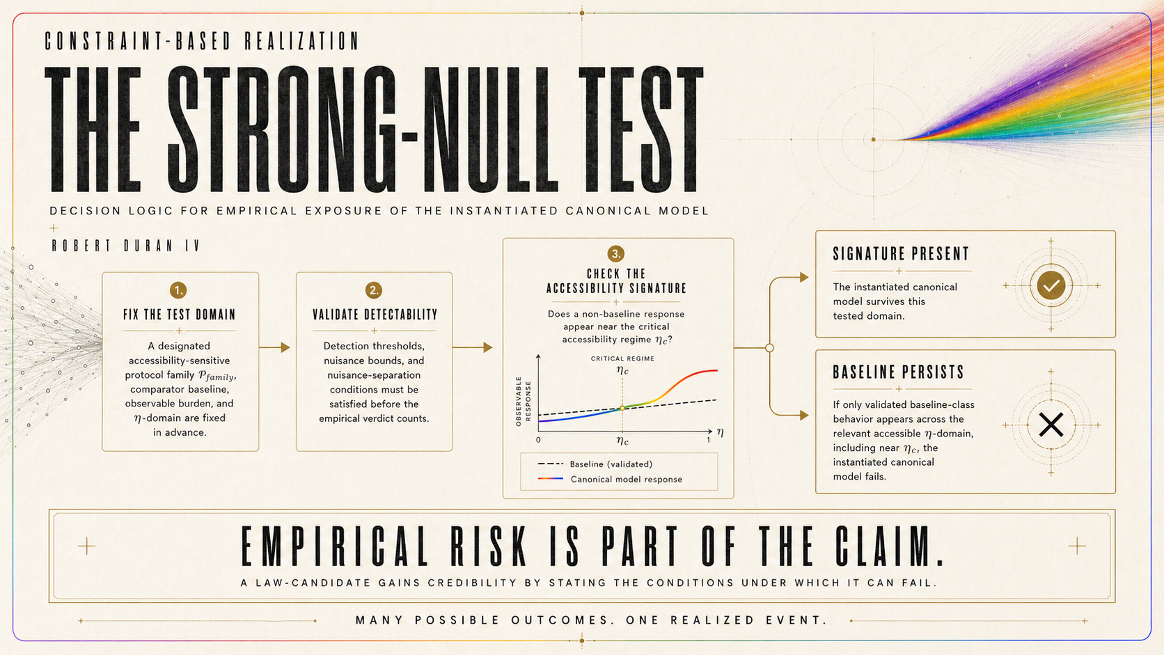
10.6. Strong-null definition
A theory candidate becomes scientifically accountable only when it states what pattern of non-observation counts against it.
Definition 10.1 (Strong null). A strong null result is obtained on the designated protocol family if, under validated accessibility calibration, validated baseline adequacy, fixed observable class, and declared nuisance model, one has
sup η ∈ I_c |V_obs(η) − V_SQM(η)| ≤ B_N + δ_exp.
This definition matters because it is stronger than merely failing to see a dramatic anomaly. A strong null is not informal absence of excitement. It is bounded non-deviation relative to the combined nuisance envelope and sensitivity floor on the exact regime where the theory says its burden must live.
10.7. Strong-null failure theorem
With the strong null defined, the failure condition for the instantiated canonical model can be stated directly.
Theorem 10.2 (Strong-null failure theorem). Assume the hypotheses of Section 9, Proposition 10.1, and the nuisance separation condition of Theorem 10.1. If a strong null result is obtained on the accessibility-critical regime I_c, then the instantiated canonical CBR model for the designated protocol family is false.
Proof. By Section 9, if accessibility enters the canonical realization law nontrivially, then the deviation amplitude on I_c is lower-bounded by L and, under the separation condition, exceeds B_N + δ_exp somewhere on I_c. A strong null states the contrary: that the observed departure from the validated baseline comparator never exceeds B_N + δ_exp anywhere on I_c. The two claims are incompatible. Therefore the instantiated canonical model is false.
Corollary 10.2 (Public failure condition). For the designated protocol family, once the nuisance envelope and sensitivity floor are validated, baseline-class behavior throughout I_c is not merely disappointing for canonical CBR. It is a failure condition for the instantiated theory.
That is the sentence that gives the paper its public experimental backbone.
10.8. Layered null taxonomy
Not every null result has the same evidential status. The paper should distinguish them explicitly.
A weak null occurs when no apparent deviation is observed, but one or more of the required calibration, nuisance-bounding, or sensitivity conditions remain incomplete. A weak null does not yet count decisively against the instantiated theory because the empirical comparison class has not been fully validated.
A strong null occurs when the designated protocol family satisfies the calibration, baseline, observable, nuisance, and sensitivity conditions of the present section, and no super-threshold departure from the nuisance baseline class appears on I_c. A strong null falsifies the instantiated canonical model under Theorem 10.2.
A framework null occurs only if it is shown that every admissible implementation of the canonical CBR law on the designated protocol family implies the same excluded deviation family. The present paper does not yet claim this strongest level globally. It states and secures the strong-null level for the instantiated canonical model.
This taxonomy is important because it prevents both overstatement and evasion. The theory is not permitted to treat every non-observation as inconclusive, and the critic is not permitted to treat every early negative result as a universal refutation without regard to calibration and nuisance validation.
10.9. Detectability budget
The final empirical ingredient is the detectability budget: the explicit condition under which the designated protocol family becomes decisively discriminating.
Let
δ_eff = δ_eff(N, σ_phi, ε_d, ε_η)
denote the effective sensitivity floor determined by sample size N, phase instability σ_phi, detector inefficiency ε_d, and accessibility-calibration uncertainty ε_η. The experiment is decisively discriminating for the instantiated canonical model if
sup η ∈ I_c L(η) > B_N + δ_eff.
This inequality is the operational compression of the empirical burden. It says that the theory’s lower-bound deviation must rise above both the nuisance envelope and the effective experimental floor on the accessibility-critical regime. If that condition is met and no such deviation is observed, the instantiated theory fails. If that condition is met and the deviation is observed, nuisance-distorted baseline dynamics do not explain it.
The detectability budget is therefore not ancillary engineering detail. It is the final bridge between theorem and experiment. It tells the reader exactly what kind of experimental regime would count as decisive.
10.10. What this section proves and does not prove
This section proves that the empirical burden of canonical CBR is not reducible to idealized baseline comparison alone. Once the nuisance class is bounded, the theory states a separation condition under which ordinary baseline distortions cannot mimic the canonical deviation family. It also proves that, when that separation condition is met, baseline-class behavior across the accessibility-critical regime constitutes a strong null and therefore a failure condition for the instantiated canonical theory.
This section does not yet prove that every conceivable implementation of the protocol family in every future platform yields the same numerical nuisance envelope or the same exact lower-bound function. Nor does it establish a universal framework-null theorem spanning all admissible extensions of the theory. Those stronger burdens remain separate.
What this section does establish is the exact empirical upgrade needed here: the theory now states not only where its signature must live and when it is detectable, but also what ordinary imperfections cannot explain it and what validated null result would count against it.
10.11. Consequences for the status of the paper
With this section in place, the paper’s empirical architecture is complete at the level required for a canonical theorem paper. The theory now contains a canonical realization law, an admissibility-restricted channel class, a locally closed weighting structure, an operational accessibility parameter, a designated protocol family, a bounded accessibility-signature regime, a detectability threshold, a nuisance separation theorem, and a strong-null failure condition.
That is a materially stronger position than a merely interpretive or suggestive proposal. The paper no longer says simply that the law might one day be tested. It states the bounded regime in which the test must matter, the conditions under which ordinary imperfections do not explain the result, and the validated null pattern under which the instantiated theory fails.
11. Rival Explanations and Exclusion Analysis
The purpose of this section is not to rehearse the full interpretive literature on quantum measurement. The purpose is narrower and more exact. Once the canonical law form, the admissibility structure, the restricted uniqueness theorem, the local weighting closure, the operational accessibility variable, the designated protocol family, the bounded accessibility-signature regime, the nuisance separation condition, and the strong-null failure criterion have all been stated, the theory must show that its central claim is not trivially absorbed by the most familiar rival explanatory moves. This section therefore asks a restricted question: does the exact object defined in the preceding sections reduce without remainder to any of the leading alternative explanatory patterns? Within the scope of the present paper, the answer is no.
This negative answer is not obtained by broad metaphysical comparison. It is obtained by matching the exact burden of the canonical theory against the exact explanatory burden carried by each rival class. The issue is not whether those rivals are historically important, sophisticated, or coherent on their own terms. The issue is whether they reproduce the theorem-bearing structure of the present paper: a canonically specified realization law, an admissibility-restricted realization class, restricted uniqueness up to operational equivalence, a locally closed weighting structure inside canonical admissibility, an accessibility-sensitive empirical burden in a designated protocol family, and a public invalidation condition under validated null behavior. What follows is therefore an exclusion analysis, not a survey.
11.1. Decoherence-only baseline
A decoherence-only account does not reproduce the object defined in this paper because it does not, by itself, supply a realization law. Decoherence explains the suppression of interference in reduced subsystem descriptions, the emergence of dynamically stable record-bearing structures, and the practical inaccessibility of certain phase relations. It therefore belongs to the level of evolution and registration already distinguished earlier in the paper. What it does not by itself furnish is a law selecting one realized outcome channel from an admissible class of realization-compatible channels.
This difference is exact rather than rhetorical. The present paper introduces a context-indexed selection rule of canonical form and proves that, within the admissibility class, the selected realization channel is fixed up to operational equivalence. It then further proves that the associated local weighting structure is not freely chosen within canonical admissibility. A decoherence-only account contains no independent realization functional, no admissibility-restricted class of realization channels, no restricted uniqueness theorem for selected realization, and no local probability-closure result of the type established in Section 6. It may reproduce ordinary visibility degradation, decoherence envelopes, and conditional recovery logic in the designated protocol family. That is precisely why it serves as the baseline comparator. But it does not reproduce the law-bearing content of canonical CBR. It supplies the comparator, not the canonical object being compared.
The newer empirical structure of the paper makes this difference sharper than before. Under the present version of the theorem chain, the issue is no longer just whether a baseline decoherence account can describe smooth visibility loss and conditional reconstruction. The issue is whether it reproduces a bounded accessibility-critical regime, a lower-bound deviation structure conditional on accessibility relevance, a nuisance-separated departure class, and a strong-null failure condition for the instantiated realization law. Decoherence-only language does not supply those features because it does not posit a realization law to which accessibility can become law-level relevant in the first place. It therefore remains what it should remain: the validated baseline response class against which the theory is tested, not a reduction of the theory itself.
11.2. Collapse-style reinterpretations
Canonical CBR is not merely relabeled collapse. Collapse-style theories typically introduce, either stochastically or dynamically, a rule by which superposed state structure is interrupted, reduced, or driven toward one outcome branch. Such theories may be serious on their own terms. But they are not equivalent to the canonical form fixed in this paper.
The difference is not that one speaks of realization while the other speaks of collapse. The difference is structural. Canonical CBR is framed as a constrained law-selection problem over an admissible class of realization-compatible channels, with canonical burden terms tied to representational invariance, record-structural coherence, and accessibility consistency. The theory’s empirical burden is then routed through an operational accessibility variable and a designated protocol family. A generic collapse-style reinterpretation does not, by that fact alone, reproduce an admissibility-restricted channel class, a burden-representation theorem, a canonical representation theorem, a restricted uniqueness result up to operational equivalence, or a local no-alternative weighting theorem inside the canonical admissibility structure. Nor does generic collapse rhetoric, by itself, imply the bounded accessibility-signature architecture now stated in Sections 9 and 10.
This distinction becomes sharper once nuisance separation is included. A collapse-style theory that merely asserts single-outcome selection still owes an explanation of why the relevant empirical burden should take the bounded accessibility-sensitive form fixed here, why ordinary nuisance cannot absorb that form once the lower-bound condition is met, and why baseline-class behavior across the accessibility-critical regime would count as a public failure condition. Canonical CBR is not equivalent to “something collapse-like happens.” It is a much more restricted claim: outcome realization is selected by a canonically represented admissibility burden whose nontrivial accessibility dependence incurs a bounded experimental liability. A generic collapse label does not reproduce that structure.
11.3. Everettian absorption
An Everettian account does not absorb the exact object defined in this paper because it answers a different question. The present paper takes as its target the law by which one realized outcome structure is selected in an individual measurement context. An Everettian account typically treats the persistence of multiple effectively decohered branches as the relevant ontological outcome rather than as a situation requiring single-outcome realization law. The difference, therefore, is not merely verbal. It is target-level.
If one denies that a realized single-outcome selection law is needed, one has not reproduced canonical CBR. One has declined its explanatory target. That may be a coherent move, but it is not an absorption of the present theory. The canonical object defined here consists precisely in the claim that one realized channel is selected from an admissible class and that this selection is canonically constrained, operationally meaningful, and empirically vulnerable. An Everettian framework may reinterpret the significance of records, decoherence, and branch structure, but it does not thereby reproduce the present law-bearing object. It changes the question.
This matters especially at the empirical level. The present theory does not merely say that record structure matters. It says that operational accessibility may become realization-effective in a bounded regime and that, if it does, a non-baseline response must emerge under stated conditions. An Everettian account that remains wholly within the standard smooth-response comparator class has not absorbed that claim. It has retained the baseline and denied the law-level transition. The exclusion analysis is therefore exact: Everettian absorption does not reduce canonical CBR without remainder; it bypasses the selective target on which the theory is built.
11.4. Hidden-variable reinterpretation
Canonical CBR is also not well described as a hidden-variable theory in the usual sense. A hidden-variable framework typically attempts to supplement the standard state description with additional ontic parameters that determine measurement outcomes or trajectories more fully than the ordinary quantum state does. The explanatory form of the present paper is different. Canonical CBR does not posit a latent state variable whose value independently determines which outcome occurs. It formulates realization as a constrained selection law over an admissible channel class.
This distinction is important because the burden architecture of the present theory is not built around hidden ontic supplementation. It is built around representational invariance, admissibility restriction, record-structural coherence, accessibility consistency, and empirical exposure through a designated protocol family. Calling the theory “hidden-variable-like” risks misdescribing both its formal machinery and its explanatory target. The theory does not claim that ordinary quantum dynamics is incomplete because an unseen parameter must be attached to each system. It claims that outcome realization requires a law of admissible channel selection not reducible to ordinary evolution and not determined by descriptive accident. That is not the same explanatory form.
The empirical difference matters as well. A hidden-variable reinterpretation would still need to reproduce the specific theorem-bearing chain developed here: bounded accessibility-critical regime, lower-bound deviation structure conditional on accessibility relevance, nuisance separation above a controlled bound, and strong-null failure of the instantiated model under validated baseline-class behavior. Absent that reproduction, the label “hidden-variable” does not absorb the theory. It merely classifies it loosely by family resemblance while leaving the actual formal and empirical object untouched.
11.5. Why ordinary smooth-response baselines are insufficient
The exclusion of rival absorption is completed by the theorem structure itself. The designated protocol family already has an ordinary smooth-response comparator. That comparator includes standard quantum evolution, entanglement, decoherence accounting, and conditional reconstruction logic. If accessibility is physically irrelevant to realization, then the law collapses toward that baseline response class. If accessibility is physically relevant to realization, then the revised empirical theorems state something stronger than before: there exists a bounded accessibility-critical regime in which global baseline coincidence fails, the departure is lower-bounded in principle, and the departure becomes experimentally significant whenever the lower-bound structure rises above the nuisance envelope and effective sensitivity floor.
This point matters because many rival explanations gain apparent sufficiency only by remaining at the level of baseline behavior. Decoherence-only language, branch-conditioning language, generic collapse rhetoric, or hidden-variable relabeling may each sound adequate if the only empirical standard is whether the ordinary response can be described after the fact. The present paper imposes a stronger standard. It asks whether the exact law-bearing object it has defined leaves the baseline class in the exact protocol family where its distinctness is supposed to appear, survives nuisance separation under the stated bound, and incurs a public failure condition under strong-null behavior. If a rival account remains wholly baseline-class while the canonical law requires non-baseline response under the stated conditions, then that rival account has not absorbed the theory. It has reproduced only the comparator.
That is why ordinary smooth-response baselines are insufficient as total explanations here. They describe what happens if realization-sensitive accessibility does no law-level work. The present theory asks what follows if it does. And once the theory has specified not only the protocol family but also the bounded critical regime, the detectability threshold, the nuisance separation condition, and the strong-null failure theorem, remaining wholly within the smooth-response baseline class is no longer a neutral explanatory option. It is one side of a discriminating empirical fork.
11.6. What this section accomplishes
This section does not prove that every rival interpretation is false. It does something narrower and more relevant to the paper’s burden. It shows that the exact theorem-bearing object defined in the previous sections is not trivially reducible to the most familiar alternative explanatory patterns. Decoherence alone does not supply realization law. Collapse-style language does not reproduce the constrained admissibility and burden architecture. Everettian absorption denies the selective target rather than reproducing it. Hidden-variable language misidentifies the explanatory form of the theory. And any account that remains wholly within the ordinary smooth-response baseline class fails, by that fact, to recover the accessibility-sensitive empirical burden, nuisance-separated signature class, and strong-null failure condition of the canonical law.
What this section therefore accomplishes is precise. It prevents the strengthened middle of the paper from being neutralized by loose after-the-fact absorption into familiar categories. The theory has now become too exact for that. Once the canonical law form, admissibility restriction, local weighting closure, operational accessibility variable, designated protocol family, bounded deviation regime, nuisance separation condition, and public failure criterion are all in place, rival reduction must occur at the same level of specificity or not at all. That is the exclusion result secured here.
12. Limits of the Present Result
The preceding sections materially strengthen the status of canonical CBR. The paper now specifies a canonical realization law, restricts the admissible realization class, establishes restricted uniqueness up to operational equivalence, proves local weighting closure within the canonical admissibility structure, defines an operational accessibility variable, embeds that variable in a designated protocol family, derives a bounded accessibility-signature regime, and states both a nuisance separation condition and a strong-null failure criterion for the instantiated canonical model. Those are substantial results. They do not, however, erase the limits of the present paper. The purpose of this section is to state those limits exactly.
The present work is therefore neither a claim of total interpretive closure nor a claim of universal empirical completion. It is a canonical theorem paper with explicit scope. Its value depends not on pretending to have solved every adjacent problem, but on identifying precisely what has been secured, what remains open, and why the secured results are still nontrivial.
12.1. Limits of the theorem class
The theorems proved in this paper are internal to the canonical CBR structure developed here. They establish representation, restriction, and empirical burden for the specified realization-law class under the stated admissibility axioms, regularity conditions, and protocol assumptions. They do not prove that every conceivable realization-law framework, every mathematically possible admissibility geometry, or every alternative formal reconstruction of quantum outcome selection must collapse into the same structure.
This limitation matters because the strongest imaginable version of the theory’s claim would be universal: that any physically acceptable single-outcome realization law must reduce to canonical CBR form. The present paper does not prove that. What it proves is narrower and more exact. It shows that once realization selection is constrained by operational equivalence, refinement stability, coarse-graining consistency, compositional closure, admissibility monotonicity, and the associated regularity conditions, canonical CBR form is the structural representative of realization selection within the theorem class treated here.
That is already a meaningful result. A theory candidate does not become stronger by blurring the difference between internal structural closure and universal formal inevitability. The present paper secures the former. The latter remains a broader theorem program.
12.2. Limits of accessibility reduction
The present paper defines accessibility operationally and reduces it to the control parameter η. That reduction is sufficient for the theorem-bearing structure of the paper. It is not claimed as the final or unique reduction for every future experimental implementation.
More precisely, the present work fixes accessibility through a structured operational notion involving retrieval fidelity, stability, public availability, destructive burden, and redundancy spread, then compresses that structure into a canonical scalar control parameter suitable for protocol-level discrimination. This is exactly what the current theorem sequence requires. It allows accessibility to enter the canonical burden, to generate a critical regime, and to support a designated empirical signature class.
What the paper does not prove is that the particular canonical reduction used here is the unique final reduction across every future platform, every future hardware architecture, or every future extension of the protocol family. Different experimental realizations may motivate refined accessibility maps, weighted reductions, or additional structure not needed at the canonical level of the present paper.
This is not a weakness in the present result. It is a scope condition. The paper requires accessibility to be operational enough to enter a theorem and controlled enough to support empirical discrimination. It does not require the last word on accessibility engineering across all future implementations.
12.3. Limits on probabilistic closure
The present paper now establishes a stronger result on probability than earlier versions did. Within the canonical admissibility structure, once admissible refinement, operational invariance, phase insensitivity, symmetry, normalization, nontriviality, and regularity are fixed, no distinct normalized nonquadratic weighting survives. In that exact sense, the paper achieves local probability closure for canonical CBR.
This result matters because it removes the appearance that weighting inside the canonical structure remains a matter of free design. The associated weighting rule is no longer merely chosen to recover familiar probabilistic behavior. Within the local theorem class, it is forced by refinement consistency and operational invariance.
What the paper still does not establish is the strongest possible global result. It does not prove final universal Born-neutrality closure across every conceivable realization framework or every conceivable admissibility geometry. It does not prove that every appearance of Born-type structure in quantum theory has now been derived from premises wholly external to the target weighting form. Nor does it establish that no broader noncanonical realization framework could reproduce similar local results by a different route.
Those deeper burdens remain separate. They belong to a broader theorem program concerning global probability closure rather than local closure within canonical admissibility. The present paper is therefore stronger than a compatibility argument, but narrower than a universal derivation theorem. That distinction should be preserved.
12.4. Limits of empirical scope
The empirical architecture of the paper is now substantially stronger than a general claim of testability. The theory is tied to a designated protocol family, an operational accessibility parameter, a bounded accessibility-critical regime, a lower-bound deviation structure, a detectability threshold, a nuisance separation condition, and a strong-null failure criterion for the instantiated canonical model. This is enough to make the theory empirically vulnerable in a finite and public way.
It is not, however, equivalent to universal empirical closure.
The present paper does not prove that every future implementation of the designated protocol family will yield the same numerical lower-bound function, the same nuisance envelope, or the same effective sensitivity floor. It does not establish that every experimental platform will realize the accessibility variable with the same fidelity or reduction map. It does not prove that every admissible extension of canonical CBR must generate the same exact observable shape in every optical or interferometric realization. And it does not claim that visible deviation should emerge across ordinary measurement settings in general.
The empirical claim of the paper is narrower and stronger than that. It says that for the designated protocol family, once accessibility enters the realization law nontrivially and once calibration, comparator adequacy, nuisance control, and sensitivity conditions are validated, the theory incurs a bounded empirical burden. If the relevant lower-bound departure rises above the nuisance envelope and effective detection floor, then ordinary baseline-class behavior in the accessibility-critical regime becomes a strong null against the instantiated canonical model.
That is a real empirical liability. It is not yet universal platform-independence, and it is not intended to be.
12.5. Limits of rival-exclusion scope
The exclusion analysis of the previous section is likewise restricted in scope. It shows that the exact theorem-bearing object defined in the paper is not trivially absorbed by the most familiar rival explanatory patterns. It does not prove that every alternative interpretation of quantum theory is false in all forms, nor that no future hybrid formalism could reproduce part of the present structure.
This distinction matters. The purpose of the exclusion analysis is not to eliminate the entire interpretive field. It is to prevent the specific canonical object developed here from being neutralized by loose relabeling. The paper shows that decoherence-only language does not supply realization law, that generic collapse language does not reproduce the canonical admissibility and burden architecture, that Everettian absorption bypasses the selective target rather than reproducing it, and that hidden-variable classification does not by itself capture the explanatory form of the theory. That is the relevant exclusion burden for the present work.
The broader philosophical burden of total interpretive comparison remains larger than the present paper’s aims. The paper should not claim more than this section secures.
12.6. Why the result still matters
These limits do not reduce the paper to a merely suggestive proposal. On the contrary, they clarify why the present result matters.
A weak foundational proposal usually fails in one of four ways. It never fixes a canonical law form. It never restricts the admissible realization class tightly enough to avoid arbitrariness. It never converts its probabilistic structure from preference into theorem. Or it never makes itself publicly vulnerable through a bounded empirical burden and explicit failure condition. The present paper avoids those failures.
It now does something more exact than broad interpretive advocacy. It fixes a canonical realization law, constrains admissibility, establishes restricted uniqueness up to operational equivalence, closes the local weighting burden inside the canonical class, defines accessibility operationally, places the theory into a designated protocol family, bounds the regime in which its empirical burden must live, separates that burden from ordinary nuisance under stated conditions, and specifies a strong-null failure criterion for the instantiated model.
That combination is significant even though it falls short of universal closure. The paper does not need to prove every stronger theorem in order to matter. It needs to convert a distributed research architecture into a canonically specified, mathematically constrained, finitely exposed theory candidate. That is what it now does.
12.7. Final scope statement
The correct reading of the present paper is therefore neither maximalist nor deflationary. It is not the final universal completion of every probabilistic, interpretive, and experimental burden surrounding quantum outcome selection. But neither is it merely a conceptual sketch. It occupies a narrower and more important position.
The paper secures a canonical object. It proves nontrivial structural results about that object. It ties that object to a bounded experimental liability. And it states what sort of validated null result would count against the instantiated theory. Those are exactly the marks of a serious theorem-bearing proposal.
13. Conclusion
The purpose of this paper has been to compress Constraint-Based Realization into a single canonical object: a realization-law candidate sharp enough to be mathematically constrained, operationally defined, and empirically vulnerable. In that respect, the paper has now accomplished more than a restatement of the broader CBR program. It has fixed the theory in a form that can be judged as a definite law-bearing proposal.
The paper first canonized the realization law itself. It specified a canonical selection rule over an admissible class of realization-compatible channels and thereby moved the framework beyond loose formal architecture. It then restricted that law by admissibility, showing that realization is not to be understood as an unrestricted choice over formally describable channels, but as a constrained selection problem governed by operational well-definedness, refinement stability, coarse-graining consistency, compositional closure, and admissibility separation. Within that structure, the law no longer appears merely chosen. It appears canonically represented and, under the stated regularity conditions, unique up to operational equivalence.
The paper then addressed the probabilistic burden at the level required for the canonical theory itself. Rather than leaving weighting as an internal degree of freedom, it showed that within canonical admissibility the associated normalized weighting structure is locally closed. Under admissible refinement, operational invariance, symmetry, normalization, nontriviality, and regularity, no distinct normalized nonquadratic weighting survives. This matters because it removes one of the principal remaining sources of internal looseness. Once the law form and admissibility structure are fixed, weighting is not left free as an internal design choice.
From there, the paper turned the theory outward. Accessibility was defined as an operational property of record-bearing structure and reduced to the control parameter η. That variable was not introduced as a descriptive convenience, but as the point at which realization structure becomes experimentally exposable. The theory was then embedded in a designated delayed-choice record-accessibility protocol family with a fixed baseline comparator, so that its empirical burden could no longer remain diffuse.
That burden was sharpened in exact form. The paper identified a bounded accessibility-critical regime, defined the deviation amplitude relative to the baseline comparator, derived a lower-bound deviation structure conditional on nontrivial accessibility relevance, and stated a detectability theorem for the canonical response. It then completed the empirical architecture by introducing a bounded nuisance class, proving nuisance separation, and stating the strong-null failure condition for the instantiated canonical model. At that point, the theory ceased to be merely test-oriented. It became finitely exposed.
Taken together, these results define the paper’s central achievement. It does not merely propose that outcome realization may require additional law. It specifies that law in canonical form, restricts its admissible realization class, secures restricted uniqueness, closes its local weighting burden, operationalizes the variable through which its empirical distinctiveness must appear, places it in a designated protocol family, and states the bounded conditions under which the theory is either supported or fails.
That is the correct level at which this paper should be read. Its accomplishment is not maximal closure over all foundational burdens. Its accomplishment is canonical compression. It has taken CBR from the level of distributed architecture and brought it to the level of a canonically specified, finitely exposed theory candidate.
That is a real change in status.
References
Aharonov, Y., Bergmann, P. G., and Lebowitz, J. L. “Time Symmetry in the Quantum Process of Measurement.” Physical Review 134, no. 6B (1964): B1410–B1416. DOI: 10.1103/PhysRev.134.B1410.
Bell, J. S. “On the Einstein Podolsky Rosen Paradox.” Physics Physique Fizika 1, no. 3 (1964): 195–200. DOI: 10.1103/PhysicsPhysiqueFizika.1.195.
Bell, J. S. Speakable and Unspeakable in Quantum Mechanics. Cambridge: Cambridge University Press, 1987.
Bohm, D. “A Suggested Interpretation of the Quantum Theory in Terms of ‘Hidden’ Variables. I.” Physical Review 85, no. 2 (1952): 166–179. DOI: 10.1103/PhysRev.85.166.
Bohm, D. “A Suggested Interpretation of the Quantum Theory in Terms of ‘Hidden’ Variables. II.” Physical Review 85, no. 2 (1952): 180–193. DOI: 10.1103/PhysRev.85.180.
Born, M. “Zur Quantenmechanik der Stoßvorgänge.” Zeitschrift für Physik 37 (1926): 863–867. DOI: 10.1007/BF01397477.
Born, M. “Quantenmechanik der Stoßvorgänge.” Zeitschrift für Physik 38 (1926): 803–827. DOI: 10.1007/BF01397184.
Busch, P., Lahti, P., Pellonpää, J.-P., and Ylinen, K. Quantum Measurement. Cham: Springer, 2016. DOI: 10.1007/978-3-319-43389-9.
Choi, M.-D. “Completely Positive Linear Maps on Complex Matrices.” Linear Algebra and Its Applications 10, no. 3 (1975): 285–290. DOI: 10.1016/0024-3795(75)90075-0.
Davies, E. B., and Lewis, J. T. “An Operational Approach to Quantum Probability.” Communications in Mathematical Physics 17 (1970): 239–260. DOI: 10.1007/BF01647093.
Deutsch, D. “Quantum Theory of Probability and Decisions.” Proceedings of the Royal Society of London A 455, no. 1988 (1999): 3129–3137. DOI: 10.1098/rspa.1999.0443.
Dirac, P. A. M. The Principles of Quantum Mechanics. Oxford: Oxford University Press, 1930.
Everett, H. “‘Relative State’ Formulation of Quantum Mechanics.” Reviews of Modern Physics 29, no. 3 (1957): 454–462. DOI: 10.1103/RevModPhys.29.454.
Ghirardi, G. C., Rimini, A., and Weber, T. “Unified Dynamics for Microscopic and Macroscopic Systems.” Physical Review D 34, no. 2 (1986): 470–491. DOI: 10.1103/PhysRevD.34.470.
Gleason, A. M. “Measures on the Closed Subspaces of a Hilbert Space.” Journal of Mathematics and Mechanics 6, no. 4 (1957): 885–893.
Gorini, V., Kossakowski, A., and Sudarshan, E. C. G. “Completely Positive Dynamical Semigroups of N-Level Systems.” Journal of Mathematical Physics 17, no. 5 (1976): 821–825. DOI: 10.1063/1.522979.
Griffiths, R. B. “Consistent Histories and the Interpretation of Quantum Mechanics.” Journal of Statistical Physics 36 (1984): 219–272. DOI: 10.1007/BF01015734.
Holevo, A. S. Probabilistic and Statistical Aspects of Quantum Theory. Amsterdam: North-Holland, 1982.
Joos, E., Zeh, H. D., Kiefer, C., Giulini, D. J. W., Kupsch, J., and Stamatescu, I.-O. Decoherence and the Appearance of a Classical World in Quantum Theory. 2nd ed. Berlin: Springer, 2003.
Kim, Y.-H., Yu, R., Kulik, S. P., Shih, Y. H., and Scully, M. O. “Delayed ‘Choice’ Quantum Eraser.” Physical Review Letters 84, no. 1 (2000): 1–5. DOI: 10.1103/PhysRevLett.84.1.
Kochen, S., and Specker, E. P. “The Problem of Hidden Variables in Quantum Mechanics.” Journal of Mathematics and Mechanics 17, no. 1 (1967): 59–87.
Kraus, K. States, Effects, and Operations: Fundamental Notions of Quantum Theory. Lecture Notes in Physics 190. Berlin: Springer, 1983. DOI: 10.1007/3-540-12732-1.
Lindblad, G. “On the Generators of Quantum Dynamical Semigroups.” Communications in Mathematical Physics 48 (1976): 119–130. DOI: 10.1007/BF01608499.
Lüders, G. “Über die Zustandsänderung durch den Meßprozeß.” Annalen der Physik 443, no. 5–8 (1950): 322–328. DOI: 10.1002/andp.19504430510.
Ma, X.-S., Kofler, J., and Zeilinger, A. “Delayed-Choice Gedanken Experiments and Their Realizations.” Reviews of Modern Physics 88, no. 1 (2016): 015005. DOI: 10.1103/RevModPhys.88.015005.
Nielsen, M. A., and Chuang, I. L. Quantum Computation and Quantum Information. 10th anniversary ed. Cambridge: Cambridge University Press, 2010.
Omnès, R. “Consistent Interpretations of Quantum Mechanics.” Reviews of Modern Physics 64, no. 2 (1992): 339–382. DOI: 10.1103/RevModPhys.64.339.
Schlosshauer, M. Decoherence and the Quantum-to-Classical Transition. Berlin: Springer, 2007. DOI: 10.1007/978-3-540-35775-9.
Scully, M. O., and Drühl, K. “Quantum Eraser: A Proposed Photon Correlation Experiment Concerning Observation and ‘Delayed Choice’ in Quantum Mechanics.” Physical Review A 25, no. 4 (1982): 2208–2213. DOI: 10.1103/PhysRevA.25.2208.
Spekkens, R. W. “Contextuality for Preparations, Transformations, and Unsharp Measurements.” Physical Review A 71, no. 5 (2005): 052108. DOI: 10.1103/PhysRevA.71.052108.
Stinespring, W. F. “Positive Functions on C*-Algebras.” Proceedings of the American Mathematical Society 6, no. 2 (1955): 211–216.
von Neumann, J. Mathematical Foundations of Quantum Mechanics. Translated by R. T. Beyer. Princeton: Princeton University Press, 1955. Original German edition published 1932.
Wallace, D. “Everettian Rationality: Defending Deutsch’s Approach to Probability in the Everett Interpretation.” Studies in History and Philosophy of Modern Physics 34, no. 3 (2003): 415–438. DOI: 10.1016/S1355-2198(03)00036-4.
Wheeler, J. A., and Zurek, W. H., eds. Quantum Theory and Measurement. Princeton: Princeton University Press, 1983.
Zeh, H. D. “On the Interpretation of Measurement in Quantum Theory.” Foundations of Physics 1 (1970): 69–76. DOI: 10.1007/BF00708656.
Zurek, W. H. “Decoherence, Einselection, and the Quantum Origins of the Classical.” Reviews of Modern Physics 75, no. 3 (2003): 715–775. DOI: 10.1103/RevModPhys.75.715.
Zurek, W. H. “Environment-Assisted Invariance, Entanglement, and Probabilities in Quantum Physics.” Physical Review Letters 90, no. 12 (2003): 120404. DOI: 10.1103/PhysRevLett.90.120404.
Theorem Spine
The canonical theory developed in this paper is closed by three theorems. Together they exhaust the burden claimed at the level of the present work. Their order is logically necessary. A realization-law proposal must first show that its law form selects non-arbitrarily within a restricted admissible class. It must then show that, if accessibility is realization-effective, the resulting response cannot remain globally contained within the declared standard baseline class. It must finally state the exact condition under which failure of that response burden counts against the theory itself. The present paper is organized to satisfy exactly those three burdens.
Theorem 1 — Restricted Canonical Uniqueness.
Let C be a physically specified measurement context and let 𝒜(C) be the restricted admissible class of realization-compatible channels defined by dynamical compatibility, representational invariance, record-structural coherence, accessibility consistency, and restricted probabilistic discipline. Let the canonical realization functional be
ℛ_C(Φ) = α Ξ_C(Φ) + β Ω_C(Φ) + γ Λ_C(Φ),
with α, β, γ ≥ 0 fixed. Under the stated existence and regularity assumptions, the selected realization channel
Φ*_C = argmin{ℛ_C(Φ) : Φ ∈ 𝒜(C)}
exists and is unique up to operational equivalence within 𝒜(C). Hence the canonical law does not merely constrain realization; it selects a unique physical verdict class modulo operationally null reformulation.
Theorem 2 — Accessibility-Signature Theorem.
Let 𝒫_family be the designated accessibility-sensitive protocol family and let η ∈ [0,1] be the operational accessibility parameter associated with contexts in 𝒫_family. If accessibility enters the canonical realization law nontrivially through the accessibility-consistency burden Λ_C, then the induced realization-sensitive response cannot remain globally contained in the declared smooth baseline class across the full admissible η-domain. Under the strongest regularity assumptions, the resulting non-equivalence is localized near a critical accessibility value η_c and appears as a critical-regime derivative break or kink in the primary observable. If those stronger regularity assumptions are relaxed while the accessibility-sensitive transition remains nontrivial, a bounded non-baseline deviation class persists in a nonempty neighborhood of η_c. Hence the theorem fixes both the regime and the admissible form of the theory’s first empirical manifestation.
Theorem 3 — Failure Criterion.
Let the canonical law form, the admissibility structure, the operational accessibility parameter η, the designated protocol family 𝒫_family, the baseline comparator, and the observable burden all be fixed exactly as stated in this paper. If 𝒫_family, under detectability-valid conditions, exhibits only baseline-class behavior across the physically relevant and experimentally accessible η-domain, with neither the strong-form nor weak-form accessibility signature appearing beyond the declared tolerance, then canonical CBR in its present form is false. Hence the theory stands not merely under comparative interpretation, but under a finite public invalidation condition.
These three theorems exhaust the burden claimed by the canonical paper. The first fixes the law as a genuine selection rule within a restricted admissible class. The second fixes the exact empirical regime and admissible response class in which the law becomes observable if accessibility is realization-effective. The third fixes the exact condition under which absence of that response counts as failure of the theory. No weaker sequence would render the canonical law scientifically vulnerable, and no further theorem is required to state the paper’s present empirical standing. Nothing essential to the empirical status of the canonical model lies outside this sequence. In that sense, the theorem spine closes the paper as a testable realization-law theory candidate.
Appendix A — Formal Proof Architecture and Dependency Discipline
A.1. Purpose and scope
This appendix makes explicit the proof architecture of the paper. It does not introduce a new physical postulate, a new realization law, or a new empirical protocol. Its function is disciplinary: to separate definitions from assumptions, assumptions from theorems, representation claims from uniqueness claims, and empirical exposure from universal closure.
The main body develops canonical CBR as a realization-law framework. The appendix clarifies how the central claims depend on named assumptions. It is designed to make the theory critic-readable: a reader should be able to identify exactly what is proved, what is conditional, and what remains an extension target.
The proof architecture of the paper proceeds in the following order:
formal objects → operational equivalence → admissible class → admissibility ordering → burden representation → canonical representation → restricted uniqueness → local probability closure → operational accessibility → empirical signature → nuisance separation → strong-null failure
No later claim should be read independently of the assumptions that support it.
A.2. Formal objects and notation
Let H denote the Hilbert space associated with the physical degrees of freedom relevant to a measurement context.
Let D(H) denote the set of density operators on H.
Let C denote a physically specified measurement context. A context is not merely an observable label. It includes the measurement architecture, record-bearing structure, timing relations, and accessibility-relevant physical conditions.
Let A(C) denote the admissible class of realization-compatible channels associated with context C.
A candidate channel Phi ∈ A(C) is a physically permissible realization-channel candidate relative to C.
Let R_C denote the realization functional defined over A(C). The value R_C(Phi) represents the realization burden associated with Phi in context C.
The selected channel is denoted Phi*_C. It is chosen as the minimizer of R_C over A(C).
For website-safe notation, this can be stated in prose:
Phi*_C is the admissible realization channel that minimizes R_C over A(C).
Let Min(C) denote the set of admissible minimizers:
Min(C) = {Phi ∈ A(C) : R_C(Phi) is minimal on A(C)}.
The paper’s uniqueness claim concerns Min(C) modulo operational equivalence, not syntactic identity of channel expressions.
This distinction prevents the uniqueness theorem from being misread as a claim about syntactic identity rather than operationally invariant physical selection.
A.3. Operational equivalence and quotient structure
Definition A.1 — Operational equivalence.
Two channels Φ, Ψ ∈ 𝒜(C) are operationally equivalent, written Φ ≃ₒₚ Ψ, if no admissible experiment internal to context C distinguishes them at the level relevant to realization selection.
Operational equivalence is weaker than formal equality and stronger than notational resemblance. Two channels may be written differently while remaining operationally equivalent. Conversely, two formally similar expressions may be operationally distinct if they generate different realization-relevant consequences.
Operational equivalence is assumed to satisfy:
Reflexivity:Φ ≃ₒₚ Φ.
Symmetry: if Φ ≃ₒₚ Ψ, then Ψ ≃ₒₚ Φ.
Transitivity: if Φ ≃ₒₚ Ψ and Ψ ≃ₒₚ Ω, then Φ ≃ₒₚ Ω.
These properties permit formation of the quotient:
𝒜(C)∕≃ₒₚ.
This quotient is the physically meaningful domain for restricted uniqueness. The paper does not claim that every formal representative of the selected channel is identical. It claims:
For all Φ, Ψ ∈ Min(C), Φ ≃ₒₚ Ψ.
That is the correct target. A realization law should not depend on notation, but it also should not leave multiple operationally distinct realization outcomes equally selected.
A.4. Minimal assumption sets
The central results of the paper depend on distinct assumption sets.
Canonical representation theorem
Requires:
operational well-definedness;
non-vacuity of 𝒜(C);
coarse-graining consistency;
refinement stability;
compositional consistency;
label invariance;
admissibility separation;
burden monotonicity;
minimal admissibility burden;
finite or suitably regular quotient structure.
Restricted uniqueness theorem
Requires all assumptions of the canonical representation theorem plus:
attainment of the minimum;
no flat inequivalent minimal-burden degeneracy;
strict separation of operationally inequivalent minimizers.
Local probability-closure theorem
Requires:
phase insensitivity;
admissible refinement consistency;
permutation symmetry;
operational invariance;
normalization;
nontriviality;
regularity.
Generalized weighting uniqueness theorem
Requires the broader assumptions stated in Appendix B:
phase insensitivity;
refinement consistency;
coarse-graining consistency;
permutation symmetry;
operational invariance;
normalization;
nontriviality;
regularity;
non-circular admissibility.
Accessibility-signature theorem
Requires:
operational accessibility parameter η;
accessibility-critical regime I_c;
designated protocol family;
fixed baseline comparator V_SQM(η);
nontrivial accessibility relevance.
Detectability theorem
Requires:
lower-bound deviation function L(η);
effective sensitivity floor δ_eff.
Nuisance separation theorem
Requires:
bounded nuisance class 𝓝;
nuisance envelope B_𝓝;
lower-bound deviation structure;
effective sensitivity floor.
Strong-null failure theorem
Requires:
nuisance separation;
validated baseline adequacy;
validated accessibility calibration;
observable fixation;
strong-null observation across I_c.
No theorem in the paper should be read as stronger than its assumption set.
A.5. Representation, existence, and uniqueness
A common source of confusion is the difference between representation, existence, and uniqueness. The paper separates them.
A representation theorem states that any realization law satisfying the admissibility axioms can be expressed in canonical burden-minimization form.
An existence claim states that the burden actually attains a minimum in the relevant admissible class.
A restricted uniqueness claim states that all minimizers are operationally equivalent.
The logical order is:
admissibility structure → canonical representation → attainment → restricted uniqueness.
Canonical representation alone does not prove strict uniqueness. Existence alone does not prove uniqueness. Restricted uniqueness requires both existence and exclusion of operationally inequivalent minimizers.
This distinction prevents overclaiming. The paper does not say that canonical form alone establishes ontological inevitability. It says that, within the theorem class, admissible realization selection is representable in canonical form, and under additional regularity conditions the selected realization channel is unique up to operational equivalence.
A.6. Admissibility axioms and regularity conditions
The canonical theorem class depends on the following axioms.
A1. Operational well-definedness.
Realization selection must be invariant under operationally equivalent descriptions of the same physical context.
A2. Non-vacuity.
For every admissible context C, the class 𝒜(C) is nonempty.
A3. Coarse-graining consistency.
If C′ is a coarse-graining of C, then selection in C must induce an admissible selected structure in C′.
A4. Refinement stability.
If C′ refines C, then the selected structure in C must be recoverable from the selected structure in C′.
A5. Compositional consistency.
Independent subcontexts must yield compatible joint and factorwise selections.
A6. Label invariance.
The realization law may not depend on relabelings with no operational content.
A7. Admissibility separation.
Operationally inequivalent candidates must remain distinguishable at the level relevant to realization selection.
A8. Burden monotonicity.
A less admissible candidate may not be preferred over a more admissible candidate.
A9. Minimal admissibility burden.
The selected channel is selected by minimal admissibility burden over 𝒜(C).
The restricted uniqueness theorem additionally uses:
R1. Attainment.
The burden ℛ_C attains its minimum on 𝒜(C).
R2. No flat inequivalent degeneracy.
Minimal-burden plateaus do not contain multiple operationally inequivalent channel classes.
R3. Strict separation.
Operationally inequivalent candidates are separated strongly enough to prevent unresolved minimal-burden collapse.
The axioms define the admissible theorem class. The regularity conditions convert canonical representation into restricted uniqueness.
A.7. Semi-formal proposition chain
Proposition A.1 — Operational quotient well-definedness
Under A1 and A6, realization selection descends to the quotient 𝒜(C)∕≃ₒₚ.
Proof. If two admissible channel candidates differ only by operationally irrelevant representation or label, then selecting differently between them would violate operational well-definedness or label invariance. Therefore the law is well-defined on operational equivalence classes.
Proposition A.2 — Admissibility preorder well-definedness
Under A1–A8, admissibility induces a preorder ≼₍C₎ on 𝒜(C)∕≃ₒₚ.
Proof. Burden monotonicity supplies the ordering direction. Operational quotienting removes representation-sensitive distinctions. Coarse-graining, refinement, composition, and label invariance ensure stability of the ordering under admissibility-preserving transformations. The induced relation is reflexive and transitive, hence a preorder.
Proposition A.3 — Order representability
Under A1–A8 and finite or suitably regular quotient structure, the admissibility preorder admits a scalar burden representation ℛ_C, unique up to order-preserving reparameterization.
Proof. On a finite quotient, every preorder admits a numerical representation by assigning values compatible with the ordering. In suitably regular infinite settings, additional topological assumptions are required. The burden ℛ_C represents the admissibility order by assigning lower burden to no-less-admissible classes.
Proposition A.4 — Affine-renormalization invariance
If ℛ′_C(Φ) = aℛ_C(Φ) + b with a > 0, then ℛ_C and ℛ′_C select the same minimizers over 𝒜(C).
Proof. Positive affine transformation preserves ordering. Since minimization depends only on order, the minimizing class is unchanged.
Proposition A.5 — Canonical representation
Under A1–A9, any realization law satisfying the admissibility structure is representable in canonical CBR form up to operational equivalence and burden renormalization.
Proof. A1–A8 yield a well-defined admissibility preorder over the operational quotient and a scalar burden representation. A9 identifies selected realization with minimal admissibility burden. Proposition A.4 ensures that positive affine renormalization does not change the selected class. Therefore the law is representable in canonical burden-minimization form.
Proposition A.6 — Restricted uniqueness modulo operational equivalence
Under A1–A9 and R1–R3, the selected realization channel is unique up to operational equivalence.
Proof. R1 gives existence of at least one minimizer. R2 excludes minimal-burden plateaus containing multiple operationally inequivalent classes. R3 ensures that operationally inequivalent minimizers cannot remain unresolved by the admissibility structure. Therefore all minimizers lie in one operational equivalence class.
A.8. Finite-dimensional scope and extension burden
The paper’s theorem class is stated in finite-dimensional or suitably regular settings.
This is a scope condition, not a defect. The designated protocol family can be modeled through finite-dimensional effective truncations or finite-dimensional operational reductions. In such settings, quotient construction, order representation, and minimization are mathematically controlled.
An infinite-dimensional extension would require additional assumptions, including:
compactness or effective compactness of the admissible set;
lower semicontinuity of the burden functional;
domain control for unbounded operators;
stability of operational equivalence classes under limits;
existence of minimizers or approximate minimizers;
continuity of refinement and coarse-graining maps;
preservation of admissibility under limiting procedures.
The present paper does not claim to have completed that extension. It establishes canonical representation and restricted uniqueness in the finite-dimensional or suitably regular theorem class required for the core paper.
A.9. Proof pressure points
The most likely critical pressure points are explicit.
Operational equivalence
A critic may ask whether ≃ₒₚ is too coarse or too permissive. The paper treats it as a named relation rather than an informal similarity claim.
Admissibility preorder
A critic may ask whether admissibility really induces an order. The paper makes this conditional on burden monotonicity and admissibility stability.
Order representation
A critic may challenge scalar representation. The paper confines the result to finite or suitably regular quotient structures.
No-flat-degeneracy
A critic may argue that uniqueness is assumed. The paper therefore states R2 explicitly and restricts the uniqueness theorem accordingly.
Local probability closure
A critic may suspect covert insertion of quadratic weighting. The paper separates local closure from universal closure and uses refinement consistency, operational invariance, and regularity rather than definitional insertion.
Empirical calibration
A critic may argue that empirical failure cannot be decisive without calibration. The paper distinguishes weak nulls from strong nulls and requires validated calibration, nuisance bounds, and sensitivity.
These pressure points are not hidden. They are the exact locations where the theorem class is conditional.
A.10. Failure diagnostics
Each assumption blocks a specific failure mode.
If operational well-definedness is removed, realization can depend on presentation rather than physics.
If non-vacuity is removed, the law may select over an empty admissible class.
If coarse-graining consistency is removed, selection can change under observational compression.
If refinement stability is removed, selection can depend on arbitrary resolution.
If compositional consistency is removed, independent systems can produce incompatible joint and factorwise selections.
If label invariance is removed, relabeling can generate artificial outcomes.
If admissibility separation is removed, distinct candidates can collapse into a trivial class.
If burden monotonicity is removed, the law may prefer less admissible candidates.
If minimal burden selection is removed, admissibility no longer determines realization.
If attainment is removed, a minimum may not exist.
If nondegeneracy is removed, multiple inequivalent minima may remain.
If strict separation is removed, operationally distinct minima may not be distinguishable by the selection structure.
If phase insensitivity is removed, weighting may depend on physically irrelevant phase labels.
If refinement consistency is removed, branch splitting may change probability.
If operational invariance is removed, representation may change probability.
If normalization is removed, weighting no longer defines probability.
If regularity is removed, pathological additive solutions may enter.
If accessibility calibration is removed, η cannot function as an empirical control variable.
If baseline adequacy is removed, deviation from the comparator loses interpretive force.
If bounded nuisance is removed, ordinary imperfections can absorb the predicted signature after the fact.
If sensitivity validation is removed, absence of observed deviation cannot count as a strong null.
The assumptions are not decorative. Each prevents a definite collapse mode.
A.11. Established, conditional, and open claims
Established in this paper
The paper establishes a canonical realization-law form over an admissible realization-channel class.
It establishes canonical representation under stated admissibility axioms.
It establishes restricted uniqueness up to operational equivalence under stated regularity assumptions.
It establishes local probability closure within canonical admissibility.
It establishes operational accessibility and a designated protocol family.
It establishes a bounded accessibility-signature regime, nuisance separation structure, and strong-null failure condition for the instantiated canonical model.
Conditional on stated assumptions
Canonical representation is conditional on A1–A9 and suitable quotient regularity.
Restricted uniqueness is conditional on R1–R3.
Local probability closure is conditional on the weighting assumptions.
Empirical exposure is conditional on calibration, baseline adequacy, nuisance bounds, and sensitivity validation.
Not established here
The paper does not establish universal closure over every possible realization-law alternative.
It does not establish final universal Born-neutrality closure across all admissibility geometries.
It does not establish universal platform-independence of the empirical signature.
It does not establish framework-null closure for all future versions of CBR.
Extension targets
A fully general representation theorem beyond finite-dimensional or suitably regular settings.
A global probability-closure theorem beyond the assumptions of Appendix B.
A platform-specific experimental model with measured values for L(η), B_𝓝, and δ_eff.
A framework-null theorem covering all admissible future implementations.
A.12. Reading discipline
The results should be read in this order:
First, as a conditional canonical representation theorem.
Second, as a restricted uniqueness theorem modulo operational equivalence.
Third, as a local weighting-closure theorem inside canonical admissibility.
Fourth, as a generalized weighting uniqueness theorem under Appendix B’s assumptions.
Fifth, as an empirical exposure claim for an instantiated protocol family.
Reading the later claims as assumption-free universal theorems would be incorrect. Reading them as merely interpretive would also be incorrect.
The correct reading is intermediate and stronger: the paper establishes a canonically specified, assumption-tracked, locally probability-closed, and finitely exposed realization-law candidate.
A.13. Why Appendix A matters
Appendix A makes the proof chain inspectable. It shows that the paper’s claims are not scattered assertions, but a structured theorem chain with named assumptions, regularity conditions, pressure points, and failure diagnostics.
That is what makes the framework critic-readable.
Appendix B — Weighting Uniqueness and the Structural Cost of Nonquadratic Alternatives
B.1. Purpose and scope
Section 6 proves local probability closure inside canonical CBR. It shows that within the canonical admissibility structure, the normalized weighting rule is not free: admissible refinement, operational invariance, symmetry, normalization, nontriviality, and regularity force quadratic modulus weighting.
This appendix strengthens that result. It asks whether the quadratic rule follows only from the specific canonical burden architecture of CBR, or whether it follows from a broader class of admissible weighting frameworks. The result is a generalized weighting uniqueness theorem.
The central claim is:
Any admissible weighting framework must either reduce to quadratic weighting or reject at least one structurally serious requirement.
This does not prove final universal Born-neutrality closure. It does prove that nonquadratic alternatives are not free. They must pay a visible structural price.
B.2. Generalized admissible weighting frameworks
Let an admissible decomposition be:
ψ = ∑ᵢ αᵢ eᵢ.
Here eᵢ denotes an outcome-defining component in an admissible decomposition class, and αᵢ is its complex amplitude.
A generalized weighting rule W assigns a nonnegative weight to branch amplitude α.
A framework is a generalized admissible weighting framework if:
branch amplitudes are defined relative to an admissible decomposition class;
branch weights are nonnegative;
refinement and coarse-graining operations are available;
operationally equivalent decompositions induce equivalent weights;
normalized total weight is well-defined.
This definition is broader than canonical CBR. It does not presuppose ℛ_C, 𝒜(C), or channel minimization. It isolates the weighting structure itself.
B.3. Structural assumptions B1–B9
B1. Phase insensitivity.
For every phase θ:
W(α) = W(eⁱᶿα).
B2. Refinement consistency.
If α is refined into admissible subbranches α₁, …, αₘ satisfying
∑ⱼ │αⱼ│² = │α│²,
then
W(α) = ∑ⱼ W(αⱼ).
B3. Coarse-graining consistency.
If admissible subbranches are aggregated into a parent branch preserving squared modulus, total weight is preserved.
B4. Permutation symmetry.
Equal-modulus branches receive equal weight.
B5. Operational invariance.
Operationally equivalent decompositions induce the same normalized weighting.
B6. Normalization.
For normalized decompositions:
∑ᵢ W(αᵢ) = 1.
B7. Nontriviality.
Unequal amplitudes are not forced into branch-count uniformity.
B8. Regularity.
W is measurable or continuous as a function of │α│.
B9. Non-circular admissibility.
Refinement and coarse-graining are not defined by secretly assuming the target quadratic weighting rule.
B.4. Why B1–B9 are structurally serious
These assumptions are not arbitrary conveniences.
Rejecting phase insensitivity permits probability to depend on physically irrelevant phase labels.
Rejecting refinement consistency permits branch splitting to alter probability.
Rejecting coarse-graining consistency permits aggregation to alter probability.
Rejecting permutation symmetry permits labels to matter.
Rejecting operational invariance permits representation to change probability.
Rejecting normalization forfeits probability interpretation.
Rejecting nontriviality preserves branch-count uniformity only by evading unequal-amplitude structure.
Rejecting regularity admits pathological additive functions with no clear physical interpretation.
Rejecting non-circular admissibility makes the theorem vacuous by hiding the conclusion in the premise.
Thus B1–B9 are not merely sufficient assumptions. They are structural requirements any physically serious weighting framework must either accept or openly reject.
B.5. Additive measure representation theorem
By B1, weighting depends only on modulus. Hence there exists f such that:
W(α) = f(│α│).
Define:
g(x) = f(√x).
Theorem B.1 — Additive measure representation.
Under B1–B5, the weighting rule induces a finitely additive nonnegative measure over admissible branch-refinement classes.
Proof. Phase insensitivity reduces weighting to modulus. Refinement consistency preserves total weight under branch subdivision. Coarse-graining consistency preserves total weight under aggregation. Permutation symmetry removes label dependence. Operational invariance ensures equivalent decompositions receive equivalent weighting. Therefore weight descends to an additive measure over admissible refinement classes.
The result is that weighting is no longer an arbitrary branch assignment. It is an additive measure on squared-modulus refinement structure.
B.6. Additivity on squared modulus
From the additive measure representation, for admissible x, y ≥ 0 with x + y ≤ 1:
g(x + y) = g(x) + g(y).
Proof. Let │α│² = x + y, and refine α into α₁ and α₂ such that │α₁│² = x and │α₂│² = y. Refinement consistency gives:
W(α) = W(α₁) + W(α₂).
Using W(α) = f(│α│) and g(x) = f(√x) gives:
g(x + y) = g(x) + g(y).
B.7. Linear solution under regularity
If g : [0, 1] → ℝ≥0 satisfies
g(x + y) = g(x) + g(y)
for admissible x, y ≥ 0 with x + y ≤ 1, and if g is measurable or continuous, then:
g(x) = cx
for some c ≥ 0.
This is the standard regular additive functional equation on a bounded interval. Regularity excludes pathological nonlinear solutions.
B.8. Flagship theorem: generalized weighting uniqueness
Theorem B.2 — Generalized weighting uniqueness.
Under B1–B9, the unique normalized admissible weighting rule is:
W(α) = │α│².
Proof. B1 gives modulus dependence. B2–B5 give additive measure structure. Additivity on squared modulus yields g(x + y) = g(x) + g(y). B8 gives g(x) = cx. Therefore W(α) = c│α│². B6 fixes c = 1. Hence W(α) = │α│².
B.9. Exclusion of rival weighting families
Nonquadratic power rules W(α) ∝ │α│ᵖ with p ≠ 2 fail additivity on squared modulus.
Branch-count weighting fails refinement consistency because branch number changes under admissible subdivision.
Linear modulus weighting W(α) ∝ │α│ fails squared-modulus additivity.
Ad hoc accessibility-modulated weighting W(α, η) fails unless, after normalization over admissible decompositions, it reduces to quadratic modulus weighting.
Thus the theorem excludes the most common rival families under the stated structural requirements.
B.10. Escape-route taxonomy
A nonquadratic alternative must choose one of four routes.
Physically costly escape
Reject phase insensitivity, refinement consistency, coarse-graining consistency, permutation symmetry, or operational invariance. This makes probability depend on phase labels, branch splitting, aggregation, labeling, or representation.
Mathematically pathological escape
Reject regularity. This permits pathological additive functions but sacrifices physical continuity or measurability.
Circular escape
Reject non-circular admissibility. This hides the target weighting rule in the admissibility grammar.
Non-probabilistic escape
Reject normalization. This may define some ranking or tendency, but not a probability rule.
This taxonomy is the exclusion force of the appendix. Nonquadratic alternatives are not logically impossible, but they are structurally expensive.
B.11. Near-global conclusion
Within any realization-weighting framework that preserves operational invariance, admissible refinement, coarse-graining, normalization, nontriviality, regularity, and non-circularity, quadratic modulus weighting is forced.
Any nonquadratic alternative must reject at least one physically serious structural requirement.
This is not final universal probability closure. It is a broad structural no-alternative theorem.
B.12. What remains short of final global closure
A fully global theorem would need to prove that every physically acceptable realization-weighting framework must satisfy B1–B9 or equivalent assumptions.
This appendix does not prove that final necessity claim. It proves the conditional structural result and identifies the price of escaping it.
That is the strongest safe conclusion.
B.13. Why Appendix B matters
Appendix B moves the probability result beyond canon-specific closure. It shows that quadratic weighting is not merely compatible with canonical CBR; it is forced across a broader family of admissible weighting frameworks.
The result is not universal closure, but it is a major strengthening: nonquadratic alternatives must now explain which structural requirement they abandon and why.
Appendix C — Concrete Experimental Instantiation and the Decisive Discrimination Inequality
C.1. Purpose and scope
Sections 9 and 10 define the empirical architecture of canonical CBR. They introduce operational accessibility η, critical regime I_c, baseline comparator V_SQM(η), canonical response V_CBR(η), lower-bound deviation L(η), nuisance envelope B_𝓝, sensitivity floor δ_eff, and strong-null failure.
This appendix makes that architecture concrete. It is not a lab report and does not claim measured constants. It provides a symbolic and illustrative numerical instantiation that shows how the empirical test becomes finite and calculable.
The central claim is:
The empirical burden reduces to one decisive inequality:
sup η ∈ I_c L(η) > B_𝓝 + δ_eff.
If this inequality is satisfied and the observed response remains baseline-class throughout I_c, the instantiated canonical model fails.
C.2. Minimal protocol family
The protocol family is a delayed-choice record-accessibility interferometric setup with:
a signal subsystem;
a record-bearing subsystem;
a controllable accessibility parameter η;
delayed retrieval or erasure;
a visibility-like observable V(η).
Let:
η ∈ [0, 1]
be the operational accessibility parameter.
Let:
η_c ∈ (0, 1)
be the critical accessibility value.
Let:
I_c = [η_c − ε_c, η_c + ε_c]
be the accessibility-critical interval.
Let V_obs(η) denote observed visibility, V_SQM(η) the baseline response, and V_CBR(η) the CBR response.
C.3. Baseline model
Choose the explicit baseline:
V_SQM(η) = V_max exp(−λη).
Here:
V_max ∈ (0, 1] is maximal baseline visibility;
λ ≥ 0 controls smooth baseline suppression.
This is not claimed as the unique baseline model. It is chosen because it is smooth, simple, and physically interpretable as ordinary suppression.
C.4. Threshold activation
Define the smooth threshold:
H_ε(x) = 1∕(1 + exp(−x∕ε)).
Here ε > 0 controls transition sharpness.
This avoids assuming a literal discontinuity while preserving a sharp transition near η_c.
C.5. CBR response model
Define:
V_CBR(η) = V_SQM(η) − κ H_ε(η − η_c)│η − η_c│ᵖ.
Here:
κ > 0 is accessibility-response strength;
p ≥ 1 controls growth shape;
η_c is the activation center;
H_ε turns on the response.
The sign convention is arbitrary. The empirical theory depends on deviation magnitude.
C.6. Lower-bound deviation
Define:
Δ(η) = │V_CBR(η) − V_SQM(η)│.
Then:
L(η) = κ H_ε(η − η_c)│η − η_c│ᵖ.
This is the model-level lower-bound function.
The central condition is:
sup η ∈ I_c L(η) > 0.
For decisive discrimination, this is not enough. It must exceed nuisance and sensitivity.
C.7. Nuisance envelope
Let 𝓝 be the bounded nuisance class.
Define:
B_𝓝 = sup { │V₀,ᴺ(η) − V_SQM(η)│ : η ∈ I_c, N ∈ 𝓝 }.
A conservative additive budget is:
B_𝓝 = b_phase + b_detector + b_calibration + b_background.
A root-sum-square version may be used only under independence assumptions:
B_𝓝 = √(b_phase² + b_detector² + b_calibration² + b_background²).
The additive budget is safer for a minimal proposal.
C.8. Effective sensitivity floor
Define:
δ_eff = zσ_total∕√N.
Here:
z is the significance multiplier;
σ_total is total observational uncertainty;
N is sample size.
Let:
σ_total² = σ_vis² + σ_phase² + σ_cal² + σ_det².
This separates statistical sensitivity from systematic nuisance. Increasing N reduces δ_eff, but does not automatically reduce B_𝓝.
C.9. Sampling grid and test statistic
Experiments sample finitely many accessibility values.
Choose:
η₁, η₂, …, η_m ∈ I_c.
Define:
T = maxᵢ │V_obs(ηᵢ) − V_SQM(ηᵢ)│.
This is the finite-sample version of the continuum supremum.
C.10. Flagship inequality: decisive discrimination
The protocol is decisive when:
sup η ∈ I_c L(η) > B_𝓝 + δ_eff.
Finite-sample detection requires:
T > B_𝓝 + δ_eff.
A strong null is:
T ≤ B_𝓝 + δ_eff
when the model predicts a super-threshold lower-bound deviation.
C.11. Worked illustrative numerical example
The following numbers are illustrative only. They are not reported experimental values.
Let:
η_c = 0.62
ε_c = 0.10
ε = 0.03
p = 1
V_max = 0.95
λ = 0.35
b_phase = 0.004
b_detector = 0.003
b_calibration = 0.004
b_background = 0.002
Then:
B_𝓝 = 0.004 + 0.003 + 0.004 + 0.002 = 0.013.
Let:
σ_total = 0.06
z = 2
N = 10,000
Then:
δ_eff = 2 × 0.06∕√10000 = 0.0012.
So:
B_𝓝 + δ_eff = 0.0142.
Evaluate at:
η = η_c + ε_c = 0.72.
Then:
η − η_c = 0.10.
The threshold is:
H_ε(0.10) = 1∕(1 + exp(−0.10∕0.03)) ≈ 0.966.
Case 1 — sub-decisive response
Let κ = 0.08.
Then:
L(0.72) = 0.08 × 0.966 × 0.10 = 0.0077.
Since:
0.0077 < 0.0142,
the toy protocol is not decisive in this parameter setting.
Case 2 — decisive response
Let κ = 0.18.
Then:
L(0.72) = 0.18 × 0.966 × 0.10 = 0.0174.
Since:
0.0174 > 0.0142,
the toy protocol becomes discriminating in this parameter setting.
This example shows the role of Appendix C. It does not claim that κ = 0.18 is physically measured. It shows how one determines whether a proposed implementation is decisive.
C.12. Required sample size formula
For target sensitivity δ_target, solve:
δ_eff = zσ_total∕√N ≤ δ_target.
Thus:
N ≥ (zσ_total∕δ_target)².
This makes experimental planning explicit.
For example, if z = 2, σ_total = 0.06, and δ_target = 0.001, then:
N ≥ (0.12∕0.001)² = 14,400.
C.13. Strong-null condition
A strong null occurs if:
T ≤ B_𝓝 + δ_eff
while the model predicts:
sup η ∈ I_c L(η) > B_𝓝 + δ_eff.
In that case, the observed baseline-class behavior contradicts the model’s required deviation structure.
Therefore, the instantiated canonical model fails.
C.14. Parameter-identification roadmap
A future implementation must estimate or bound:
η_c
κ
p
ε
ε_c
V_SQM(η)
B_𝓝
δ_eff
N
Without these values, the experiment may be suggestive but not decisive.
C.15. What Appendix C establishes
Appendix C establishes a concrete symbolic and numerical toy roadmap.
It supplies:
explicit baseline model;
explicit CBR response model;
explicit lower-bound function;
explicit nuisance envelope;
explicit sensitivity floor;
finite-grid statistic;
decisive inequality;
strong-null criterion;
sample-size formula.
C.16. What Appendix C does not establish
Appendix C does not report measured values.
It does not claim that the toy parameters are physically realized.
It does not replace platform-specific modeling.
It does not prove that every implementation must use the same analytic deviation profile.
C.17. Why Appendix C matters
Appendix C turns empirical exposure into a calculable task. It shows exactly what future experiments must estimate and how the strong-null logic becomes operational.
That makes the empirical burden finite, test-plannable, and non-rhetorical.
Appendix D — Failure Logic, Negative Outcomes, and Theory-Death Conditions
D.1. Purpose and scope
This appendix states the failure logic of canonical CBR.
Not every null result falsifies the theory. But a validated strong null falsifies the instantiated canonical model.
The appendix prevents two errors:
treating every negative result as total theory death;
treating every negative result as inconclusive.
The goal is disciplined falsifiability.
D.2. Fixed model ingredients
Before a decisive test, the following must be fixed:
canonical realization law;
admissible class A(C);
accessibility parameter η;
critical regime I_c;
baseline comparator V_SQM(η);
canonical response V_CBR(η);
lower-bound function L(η);
nuisance envelope B_N;
sensitivity floor δ_eff;
sampling statistic T.
If these are not fixed, the test is not yet decisive.
D.3. Pre-registration condition
Before empirical confrontation, the following must be declared:
observable class;
accessibility grid;
baseline comparator;
nuisance model;
sensitivity floor;
strong-null threshold;
analysis statistic.
This prevents post hoc escape.
A theory may be revised after failure, but it may not reinterpret a failed pre-registered test as a success by changing the target after the fact.
D.4. Negative-outcome classes
Class I — Inconclusive null
No deviation is observed, but calibration, sensitivity, nuisance modeling, or baseline adequacy is incomplete.
Effect: no decisive conclusion.
Class II — Weak negative result
No deviation is observed, and the test is reasonably designed, but the decisive inequality is not satisfied.
Effect: pressure against the implementation, but no falsification.
Class III — Strong null
No deviation is observed, and all decisiveness conditions are satisfied.
Effect: the instantiated canonical model fails.
Class IV — Repeated strong null across implementations
Multiple independent implementations produce strong nulls.
Effect: severe pressure against the canonical accessibility-signature program.
Class V — Framework null
It is shown that every admissible implementation of the broader framework requires the excluded deviation class, and experiments exclude it.
Effect: framework-level failure in the tested form.
D.5. Model invalidation theorem
Theorem D.1 — Strong-null invalidation.
If the instantiated canonical model predicts
sup η ∈ I_c L(η) > B_N + δ_eff,
but a validated strong null satisfies
T ≤ B_N + δ_eff,
then the instantiated canonical model is false.
Proof. The model predicts a super-threshold deviation somewhere in I_c. The strong null states that no such deviation occurs across the tested grid in I_c within the validated nuisance-plus-sensitivity threshold. These claims are incompatible. Therefore the instantiated model is false.
D.6. Survival map
After Class I, the theory survives unchanged.
After Class II, the tested implementation is weakened, but the model is not falsified.
After Class III, the instantiated canonical model fails.
After Class IV, the canonical accessibility-signature program is severely weakened.
After Class V, the framework fails in the tested form.
This map prevents both premature refutation and indefinite evasion.
D.7. Anti-evasion rule
After a strong null, the theory may not evade failure by:
redefining η_c post hoc;
changing the observable class post hoc;
widening the nuisance envelope post hoc;
moving to a new protocol family while claiming the old test was never relevant;
weakening L(η) after the result;
declaring every baseline-class result inconclusive.
These moves are not legitimate theory survival. They are evasion.
D.8. Legitimate revision rule
A legitimate revision is allowed only if it:
is stated before a new test;
identifies which assumption has changed;
generates a new risk-bearing prediction;
does not reinterpret the failed test as success;
preserves public falsifiability.
This permits scientific development while preventing after-the-fact immunization.
D.9. Burden-shift rule
After a weak null, the burden shifts to experimental improvement.
After a strong null, the burden shifts to revision or abandonment of the instantiated model.
After repeated strong nulls, the burden shifts to explaining why the broader framework survives.
After a framework null, the burden is no longer revision. It is abandonment of the tested framework.
D.10. Theory-death conditions
CBR dies in the tested form only if:
the required deviation class is fixed;
decisiveness conditions are met;
nuisance and sensitivity are bounded;
strong nulls repeat across independent implementations;
no admissible reformulation avoids the result without evasion;
failure generalizes across the admissible protocol class.
This is a high standard, but not an impossible one. That is the correct posture for a serious foundational theory.
D.11. Why Appendix D matters
Appendix D makes the theory’s failure logic public and disciplined.
It protects the theory from premature dismissal under weak evidence, but it also prevents the theory from escaping decisive contrary evidence.
That is what makes the framework scientifically exposed rather than merely interpretive.